1Overview of frustration and correlation
Geometric frustration in magnetism is best understood in the context of the nearest neighbour Ising antiferromagnet on a triangular lattice. Variants of this, involving triangular motifs in higher dimensions, quantum spins, and more complex interactions, define this well explored field. All these systems are ‘insulators’, with no relevant charge degrees of freedom, and the nature of spin-spin interaction is predefined (otherwise the notion of frustration itself becomes ambiguous).
Correlated systems, as we will use the term in the thesis, involve itinerant electrons. The magnetic degrees of freedom, independently present or self generated, couple to these electrons. For us the magnetic degrees of freedom will reside on a traditional ‘frustrated’ structure, but the interaction between them is not necessarily short range antiferromagnetic. In fact when the electron system is ungapped the magnetic interaction is effectively long range.
For us, the frustrated lattice mainly serves to rule out Neel order. We generally do not know the spin-spin interaction, and need to solve the electron problem ‘ab initio’ to infer the magnetic state. This is where the focus of the present thesis differs from the mainstream of frustrated magnetism.
In what follows we review, successively, some of the general features associated with frustration, correlation effects, the combination of the two, and then aspects of double perovskite and Mott phenomenology relevant for us.
1.1Geometric frustration
To introduce the notion of geometric frustration let us start with the model of Ising spins () on a lattice with nearest neighbour (NN) coupling . The Hamiltonian is given by
If the ground state corresponds to all spins parallel, with total energy , being the number of lattice sites and the number of nearest neighbours. Since is also simply the number of pair interactions, one says that in this ferromagnetic case all pairwise interactions are satisfied in the ground state.
When , one may naively expect that the ground state would correspond to all NN pairs being anti-parallel. However, in contrast to a ferromagnet, such an antiferromagnetic state may not exist for a given lattice. The existence of such a state in a lattice, with all pairwise interactions satisfied, is possible only when the lattice sites can be divided into two disjoint subsets (or sub-lattices) such that all neighbours of a site in one set belong to the other set. This is a geometric property of the lattice, and when it is satisfied we call the lattice bipartite. The nearest neighbours of a given site in such a lattice are not themselves nearest neighbours of each other, so a spin arrangement exists in which all NN pairs are anti-parallel. This state is the Neel antiferromagnet. It can occur, for example, on a square lattice Figure 1(a), and a simple cubic lattice.
Figure 1:(a) The square lattice is bipartite as we can divide it into two sub-lattices, say blue and green, where neighbours of blue are only green (and vice versa). (b) In the triangular lattice such division is not possible.
A contrast is provided by the triangular lattice Figure 1(b), where the nearest neighbours of a given site are also themselves nearest neighbours. This prevents division of the lattice into two sub-lattices, the lattice is non-bipartite. Additional examples are the face centered cubic (FCC) lattice and pyrochlore lattice. On such a lattice, it is geometrically impossible to satisfy all the pairwise interactions, i.e., to have a Neel state. This situation where not all pairwise interactions can be satisfied, due to lattice geometry, is called geometric frustration.
If not the “saturated” state, what kind of low energy magnetic configurations are available in a geometrically frustrated system? While this is a difficult question for an infinite lattice, let us look at the toy problem of three Ising spins with , Figure 2. There are six possible configurations with the lowest energy , shown in the figure, and in each of them one pair has parallel spins. With all bonds satisfied the lowest energy would have been , instead of . Besides, the three site system has 6 fold degeneracy. The degeneracy of the ground state grows with system size. The classic solution of the Ising model on a triangular lattice, by Wannier Wannier (1950) in 1950, clarified the following
The ground state energy of the antiferromagnetic triangular lattice Ising model is one third of the ferromagnetic case.
There is no singularity in the temperature derivative of the energy, i.e., specific heat, hence there is no ‘Curie point’.
There is no long range order, the system is disordered at all temperatures.
The entropy at is finite ().
Figure 2:Possible anti-parallel arrangements in a three spin system. The sites are denoted by green circles, and spins by arrows. Each configuration has two satisfied bonds (gray line) and one unsatisfied bond (thick red lines).
Three years later, Kano et al Kano & Naya (1953), showed similar results for Ising spins on a Kagome lattice. In Fig.\ref{ising-e} the total energy as function of temperature, calculated by Wannier is shown for the triangular lattice (left), while the right panel shows the Kagome result. For the ferromagnetic case, there is sharp decrease in the total energy, near a `Curie point’ where the derivative, i.e., the specific heat has a singularity. For the antiferromagnetic case, however, the energy varies slowly, so the specific heat has a broad maximum instead of any singularity.
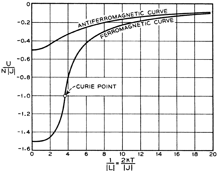

Figure 3:Temperature dependence of total energy for Ising systems. Left: Triangular lattice, from Wannier Wannier (1950). The lower(upper) curve is for ferromagnetic (antiferromagnetic) case. Right: Kagome lattice from Kano et al Kano & Naya (1953). The solid set of lower(upper) curve is for ferromagnetic (antiferromagnetic) case, while the dotted curves are corresponding triangular lattice results.
The phase diagram of the Ising model with nearest neighbour () and next neighbour () couplings, on the centered square lattice (Vacks et al. (1966), Morita et al. (1987), Morita et al. (1987)) and the Kagome lattice Azaria et al. (1987), Debauche & Diep (1992), are shown in Figure 5. The centered square lattice shows non-monotonic phase boundary, where there is a ‘reentrance’ of AF phase between ferromangetic and paramagnetic phase. In Kagome lattice, the phase boundary is between ferromagnet and a partially disordered phase, in which central spins (blue dots) are free, with bigger reentrance window. The paramagnetic phase in the Kagome lattice also has two different kind of spatial fluctuations Mézard et al., 1984 probed via a spin glass order parameter proposed in Parisi, 1983, where one calculates overlap function
and probability distribution for ,
Figure 4:The tetrahedral unit, building block of the FCC and pyrochlore lattices.
The boundary of these two disordered phases is shown by the dotted line. This line is referred to as ‘disorder line’. Reentrance, multiple thermal transition, and the presence of ‘disorder line’ has been seen in other models too. They are believed to be generic features of frustrated systems in two and three dimensions. In three dimensions for the pyrochlore or the face centered cubic (FCC) lattices the neighbouring spins live on a tetrahedral motif (Figure 4) involving four triangular faces.
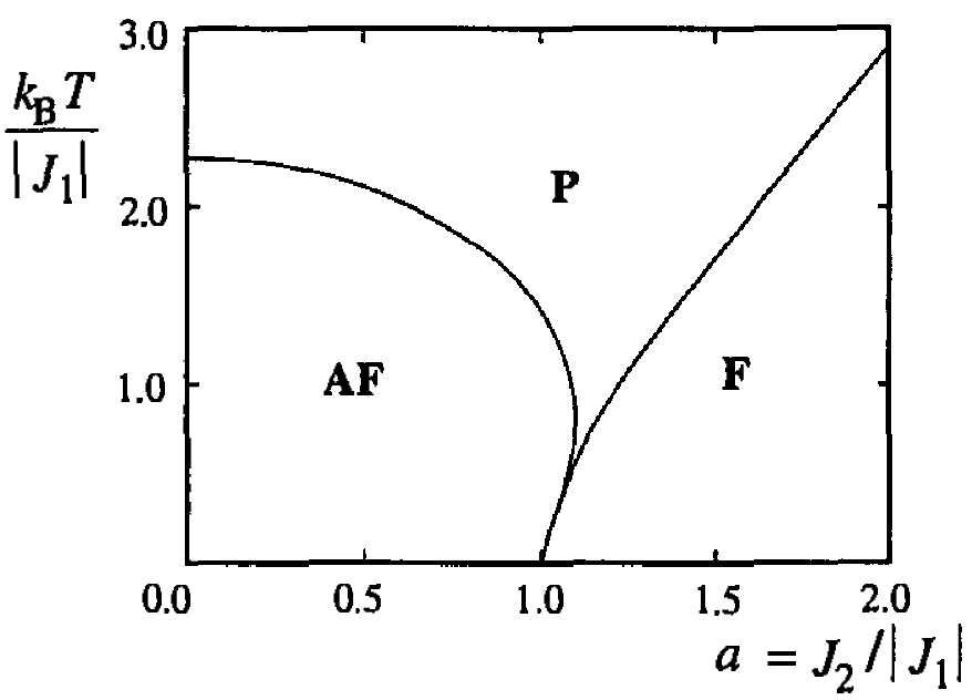
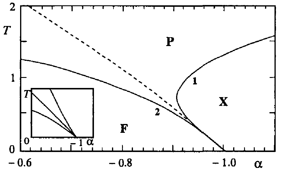
Figure 5:Temperature versus phase diagram for the antiferromagnetic Ising model on the centered square lattice (Vacks et al. (1966), Morita et al. (1987), Morita et al. (1987)) (Figure 5a) and the Kagome lattice (Azaria et al. (1987), Debauche & Diep (1992)) (Figure 5c). F, AF, P and X are respectively ferromagnet, antiferromagnet, paramagnet and partially ordered. Taken from Diep, et al Diep (2005). The structure of the lattice are shown in Figure 5b, and Figure 5d.
In case of classical Heisenberg spins (unit vectors) with AF coupling on a frustrated structure the total energy may be minimised by non-collinear or non-coplanar spin arrangements. While the Neel state cannot occur, the angular variables can allow other forms of long range order to occur. For example, on the triangular lattice one finds the well known 120 arrangement (Figure 6), and on the FCC lattice (where the ground state is actually degenerate) a ‘C-type’ phase is selected by thermal fluctuations. However, in many lattices like Kagome, checkerboard, and pyrochlore (Moessner & Chalker (1998), Moessner & Chalker (1998)), the geometric frustration is more severe, and it prevents any long range order of the AF coupled NN Heisenberg model.
In these cases, when the ground state fails to sustain long range order, it may have disordered spin arrangements, with short range AF correlations, e.g, spin glasses or spin liquids. In a spin glass, below a certain temperature referred as ‘glass transition temperature’ or ‘freezing temperature’, , the relaxation time of the spins diverges, and the spins are locked in a static random orientation. In the presence of quantum fluctuations these random orientations are no longer static, and result in spin liquid. In case of pyrochlores even the classical spins have , an unusual state referred as ‘classical spin liquid’ (Moessner & Chalker (1998), Moessner & Chalker (1998)). These situations, both in their classical and quantum versions, have been intensely studied (Diep (2005), Moessner & Chalker (1998), Moessner & Chalker (1998), Huse & Rutenberg (1992), Chalker et al. (1992)).
Figure 6:The non-collinear 120 phase.
While the triangular lattice with classical Heisenberg spins supports an ordered ground state, (Figure 6), the Kagome lattice and the pyrochlore lattice, for example, do not. In these cases the Hamiltonian can be written as a sum of squares of the total spin, , of individual units (tetrahedron in pyrochlore, and triangles in Kagome), which share only one vertex. The ground state is obtained by minimizing for every unit. This fixes relative angles within the unit but not the angles between neighbouring units, leading to a large ground state degeneracy due to this local freedom. In the Kagome lattice thermal fluctuations select a coplanar configuration (Huse & Rutenberg (1992), Chalker et al. (1992)).
What about quantum effects? For a pair of quantum spins, with AF Heisenberg coupling, the ground state is anyway not a ‘up-down’ configuration but a singlet, i.e, a specific linear combination of the ‘up-down’ and ‘down-up’ states. Consider three quantum spins on a triangle with AF Heisenberg coupling. The ground state is four fold degenerate, with energy , instead of six fold degenerate as in the classical Ising case with energy . These states are also linear combinations of ‘up-down-up’ states like , etc. In the context of a lattice, quantum fluctuations of this kind allow the system to partly overcome the loss in energy due to classical frustration.
The quantum = nearest neighbour Heisenberg antiferromagnet orders (at ) on both the square and triangular lattice (Lecheminant et al. (1997)), though the order parameter is reduced by 40% and 50% respectively, compared to the classical result. The Kagome lattice is more frustrated than the triangular lattice (Lecheminant et al. (1997), Hermele et al. (2008), Yan & others (2011), Depenbrock et al. (2012), Iqbal et al. (2013)).
Unusual ground states may also arise. The simplest object is a valence bond crystal (VBC), consisting of product of pairwise singlets of neighbouring spins (shown as cartoon in Figure 7:
In a valence bond two spins are maximally entangled. In the VBC, the state consists of static localized valence bonds, in which each spin is entangled with only one other. Several materials exhibit a VBC state (Iwase et al. (1996), Azuma et al. (1994), Kageyama & others (1999)), and are interesting as they provide an experimental way of studying Bose-Einstein condensation of magnons (which are triplet excitations of the singlet valence bonds) in the solid state. When these valence bonds are allowed to undergo quantum fluctuations, the ground state is a superposition of different pairings of spins into valence bonds (Figure 7(c)). If the distribution of these partitionings is broad, then there is no preference for any specific valence bond and the state can be regarded as a valence-bond ‘liquid’ rather than a crystal. This is generally called a resonating valence-bond (RVB) state (Anderson (1973)).
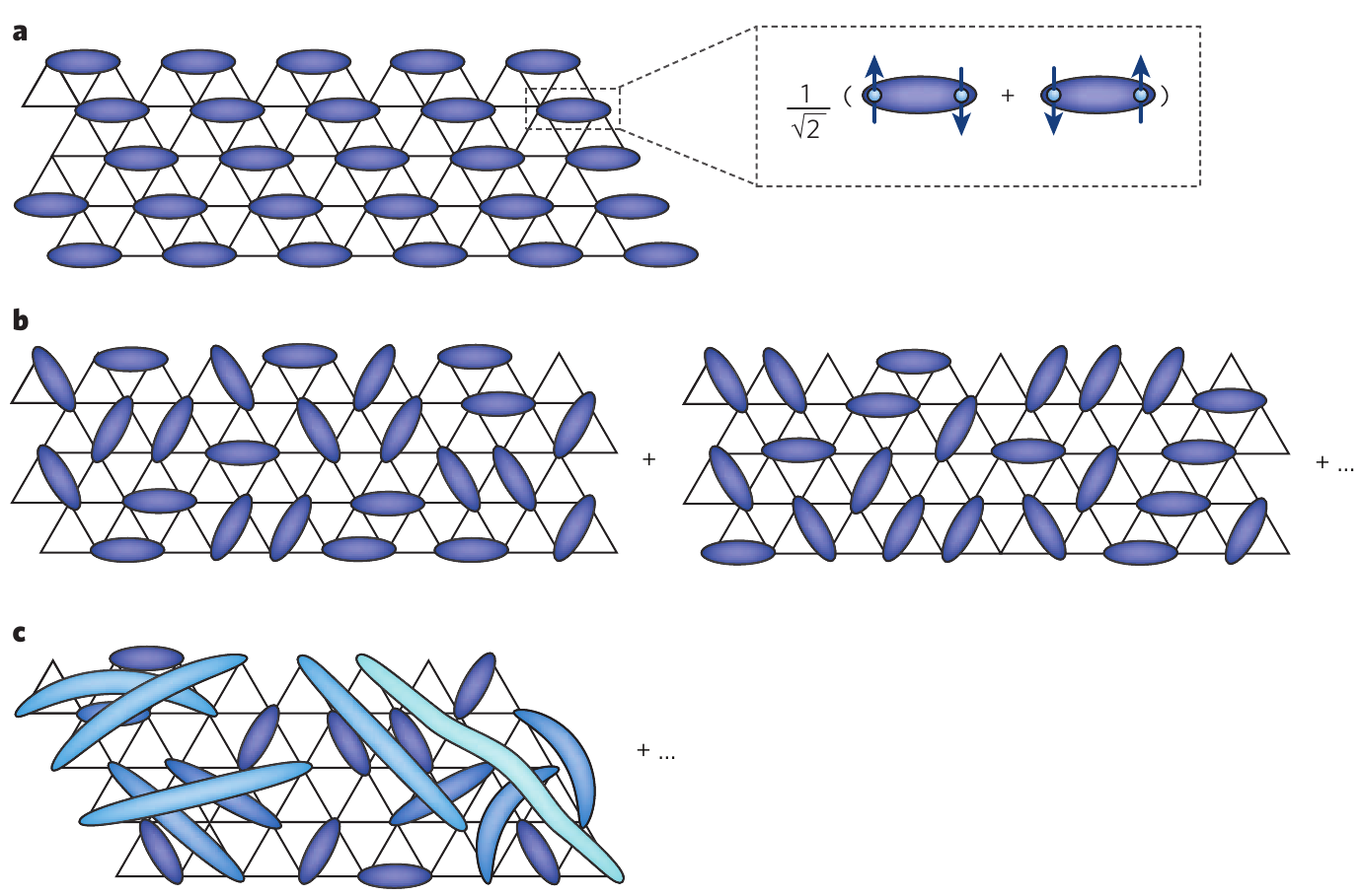
Figure 7:Cartoon of a valence bond crystal on the triangular lattice. (a) A regular arrangement of singlet bonds where blue ellipses denote the singlets. An RVB state is a superposition of many configurations of bond, which could be among (b) near neighbours, or (c) long distance apart. (From Balents \cite{frust-rev2})
The quantum Heisenberg antiferromagnet on checkerboard lattice shows long range plaquette order (Moukouri (2008), Brenig & Grzeschik (2004), Fouet et al. (2003)) at isotropic coupling while the Kagome antiferromagnetic is a spin liquid (Lecheminant et al. (1997), Hermele et al. (2008), Yan & others (2011), Depenbrock et al. (2012), Iqbal et al. (2013)).
2Electronic correlation
Electrons in a solid interact with each other and with the lattice vibrations. In case of narrow band materials, where a tight binding approximation is appropriate, short range repulsion between electrons may have important effects on electronic properties, producing magnetic moments and metal-insulator transition.
Early understanding and classification of materials in terms of their electrical character was based on band theory, where a completely filled or empty band results in insulating behaviour, while partially filled bands lead to metallic behaviour. However, it was found that several compound (e.g., NiO) do not respect this classification (Boer & Verway (1937)). Some materials, which are nominally at ‘half-filling’ behave as insulators. Peierls (Peierls (1937)) suggested that an insulating state could arise due to lattice period doubling which can arise from electron-phonon coupling induced dimerization. This could open a gap at the Fermi level.
In 1949 it was argued by Mott (Mott (1949)) that strong electron-electron interaction could prevent electron delocalisation, and lead to an insulating state, if the bandwidth fell below a critical value. This was the scenario for a Mott transition, made concrete later in terms of a minimal lattice model by Hubbard, etc.
The Hubbard model (Hubbard (1963)) (also independently conceived by Gutzwiller (Gutzwiller (1963)) and Kanamori (Kanamori (1963))) describes electron delocalisation in the presence of local repulsion. Originally introduced to address itinerant ferromagnetism (Hubbard (1963)) in transition metals, its usefulness now extends to describing metal-insulator transitions, antiferromagnetic order, and possibly -wave superconductivity. Hubbard’s several papers (Hubbard (1963), Hubbard (1963), Hubbard (1963), Hubbard (1963), Hubbard (1963)) worked out various limits of the model, and an approximate description of the Mott transition.
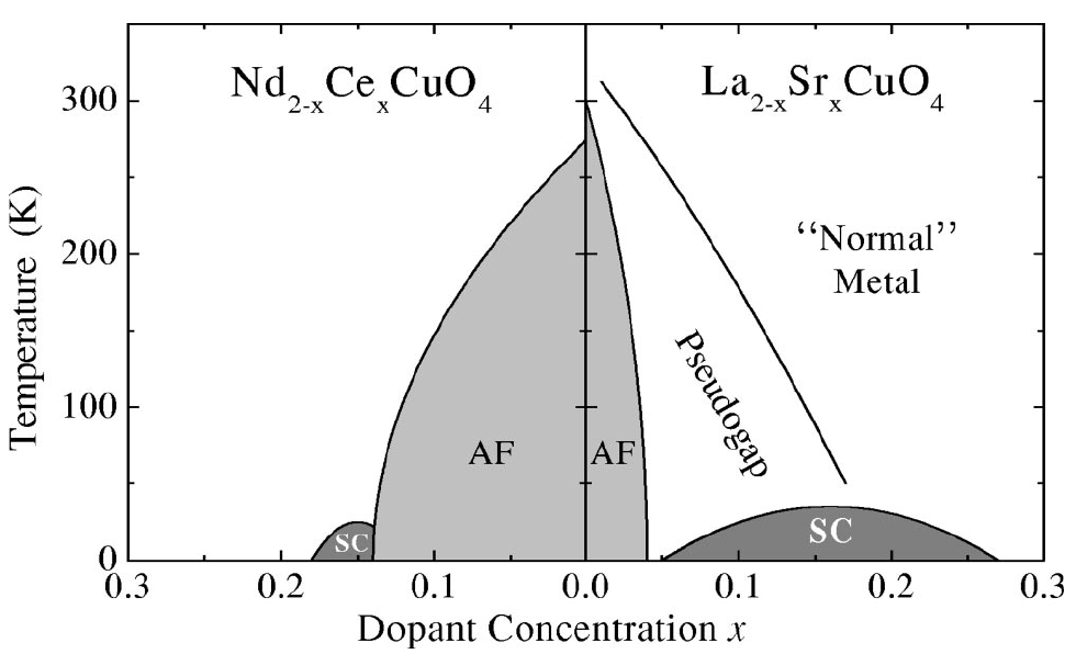
Figure 8:Phase diagram of the electron and hole doped superconductors, showing superconducting (SC), antiferromagnetic (AF), pseudogap, and normal metal regions. is the half filled Mott insulating phase. (Damascelli (Damascelli & others (2003)))
Although continuously studied since its introduction, the Hubbard model and the Mott insulator gained prominence with the discovery of high temperature superconductivity in the doped cuprate LaSrCuO (Dagotto et al. (1994), Dagotto et al. (2006), Damascelli & others (2003)). This thrust the Mott transition and the doped Mott insulator center-stage.
It quickly became apparent that a large family of transition metal oxides, including the ‘colossal’ magnetoresistance manganites (AAMnO3) (Tokura (2000), Salamon & others (2001)), the high thermopower cobaltates (NaCoO) (Lee & others (2006)), etc, owed their exotic properties to electron correlation (Anderson (1972), Fulde (1995), Fulde (2012), Fazekas (1999)).
The development of powerful tools like dynamical mean field theory (DMFT) and its combination with ab initio methods has clarified many aspects of correlation physics over the last two decades (Georges & others (1996)).
Important characteristics of these materials include: (i) the existence of several competing states, a typical example is the high phase diagram in (Figure 8), (ii) strong sensitivity to perturbations like doping change, applied fields, disorder, and temperature, and (iii) the occurence of spontaneous nanoscale inhomogeneity.
3Itinerancy and frustration
Correlation physics involves metallic systems with itinerant electrons, while traditional frustrated systems are insulating magnets with localized electrons. There are broadly two situations where they intersect:
One may have a ‘two species’ system, of electrons and local moments, where the local moments live on a frustrated structure and are Kondo (or Hund’s) coupled to itinerant electrons.
We could have a Mott insulator in a frustrated structure and the consider its metallization, due to increasing bandwidth.
The first situation arises in Kondo lattice like, or ‘double exchange’, models, while the second is described by the Hubbard model. In both cases the ideal frustrated situation arises in the absence of itinerant electrons. The interest is in clarifying how the presence of electrons in the Kondo lattice, or the approach to the insulator-metal transition in Mott-Hubbard systems modifies the physics. The ‘two species’ description is appropriate for the pyrochlores ABO (iridates, etc) and double perovskites ABBO, while the Hubbard model is relevant for materials like the cluster compound GaTaSe and AC. We review these quickly in the following sections.
4Double perovskites
4.1General introduction
The double perovskites (DP) constitute a large family of materials with the molecular formula ABBO, where A is a large electro-positive element, B and B are typically transition metals and O stands for Oxygen. They can be thought of as two units of perovskites, i.e., ABOABO. In most cases, they crystallize in alternating BO and BO octahedra arranged in the rock-salt manner, as shown in Figure 9. The physical properties of double perovskites depend on
a. The chemical combination B and B, and
b. The ionic radius and valence of A.
Figure 9:Left: The ordered double perovskite ABBO crystal structure, which consists of alternating pattern of BO, and BO octahedra, in rock-salt manner. Right: In the rock-salt B-B arrangement, each sub-lattice is FCC.
They exhibit a number of magnetic and electronic states, for example high ferromagnetic half-metal in SrFeMoO (Tomioka et al. (2000)), high ferromagnetic insulator in SrCrOsO (Krockenberger et al. (2007)), and frustrated antiferromagnetic insulators in LaLiRuO (Aharen & others (2009)). There are also exotic magnetic states like spin glass (BaYReO (Aharen & others (2010))) and valence bond glass BaYMoO (Vries et al. (2010)).
4.2Experimental results
Although studied for decades (Anderson et al. (1993), Sarma et al. (2001), Sarma et al. (2007)) it was the discovery of high ferromagnetism and half-metallicity in SrFeMoO (Kobayashi et al. (1998)) (SFMO) that led to renewed interest in the double perovskites. They display a wide variety of properties.
a. SFMO is a high T half metallic ferromagnet with moderate low field magnetoresistance. Could be useful for spintronic and switching applications.
b. LaNiMnO (Subramanian et al. (2005), Das et al. (2008)), is a ferromagnetic insulator with T, and shows large magneto-dielectric response over a window K (Choudhury et al. (2012)).
c. SrCrOsO (Krockenberger et al. (2007)) is a ferromagnetic insulator with K, with one of the highest transition temperature reported.
Table 1:List of double perovskite materials
| Perovskite | Crystal structure | Magnetism | , | Transport |
|---|---|---|---|---|
| SrFeMoO | Tetragonal | FM | 420K | Half metal |
| BaFeMoO | Cubic | FM | 345K | Half metal |
| SrFeReO | Cubic | FM | 400K | Half metal |
| SrCrReO | Cubic | FM | 635K | Half-metal |
| SrCrOsO | -- | FM | 725K | Insulator |
| CaCrReO | Monoclinic | FM | 360K | Insulator |
| CaFeReO | Monoclinic | FM | 520K | Insulator |
| LaNiMnO | Monoclinic | FM | 280K | Insulator |
| SrFeWO | -- | AF | 40K | Insulator |
| SrFeCoO | Tetragonal | SG | 75K | Insulator |
| BaYMoO | -- | VBG | 0K | Insulator |
The magnetism in the DP’s arises from a combination of Hund’s coupling on the B, B ions and electron delocalisation. While there are important DP’s where both B and B are magnetic ions e.g., LaNiMnO, we will focus on materials where only one ion, say ‘B’, is magnetic. In this category, there are insulating DP’s
(Wiebe et al. (2002), Aharen & others (2009), Aharen & others (2010), Vries et al. (2010), Gao & others (2011)), which are mostly in the category of Mott insulators, and metallic DPs, for example SrFeMoO (SFMO).
Let us focus on metallic systems, where the effect of magnetic frustration is more interesting and much less explored. A good starting point is the SFMO, where the B atom (Fe) is magnetic while B (Mo) is non-magnetic. The ferromagnetism, and its applications in SFMO is well explored (Alonso et al. (2003), Brey et al. (2006), Chattopadhyay & Millis (2001), Phillips et al. (2003), Singh & Majumdar (2011)), but much less is known about the antiferromagnetism. Recent theoretical studies predicted that upon electron doping, SFMO should show a transition to a metallic antiferromagnetic state (Sanyal & Majumdar (2009), Sanyal et al. (2009)). The synthesis of lanthanum doped (LaSrFeMoO) compounds have revealed signatures of antiferromagnetism at high doping (Jana et al. (2012)).
Figure 10:The relevant electronic levels of SrFeMoO.
The electronic structure of SFMO is shown in (Figure 10). The octahedral oxygen coordination splits the five -orbitals into a threefold degenerate lower manifold and the twofold degenerate higher energy levels. The large Hund’s splitting in Fe leads to high spin configurations, while for Mo, due to negligible Hund’s splitting the level remain almost spin degenerate. SFMO exists in the mixed valent state involving (a) Fe-Mo in which Fe has 5 electrons filled in the lower, say up spin, orbitals and Mo has 1 electron in the lowest level, and (b) Fe-Mo, in which Fe has 5 electrons in the lower up spin levels, and one electron on the next higher ‘down’ level, and Mo levels are empty.
Based on the electronic structure established by Sarma et al (Sarma & others (2000)), the lower and band of Fe lie well below the Fermi level and contribute localized spin at each Fe site, while the the upper of Fe hybridize with the corresponding of Mo. The electron hopping amplitude between the Fe, and Mo level, and the level difference are the crucial ingredients that decide the band structure of the system. The next section discusses the origin of magnetic order.
4.3Theoretical background
There have been several attempts at a theoretical understanding of the magnetism in these materials. These consist of ab initio electronic structure calculations, and model Hamiltonian based approaches.
The ab initio calculations provide material specific information about the electronic structure (Sarma et al. (2000)), relevant energy scales and couplings like the hopping , Hunds splitting and level difference (Sanyal et al. (2009)), and allow a rough mean field estimate of the (Mandal et al. (2008)). Unfortunately, these calculations are rather complicated for non-collinear magnetic phases that are likely in a frustrated magnetic lattice, which is the case for SFMO, where the localized moments lie on the FCC `B’ site sub-lattice. In such situations model Hamiltonian studies can provide some insight on possible ordered states.
The band theory for DPs like SFMO is described as sum of three two-dimensional (2D) tight binding models, involving and planes, respectively, due to three bands. On the sites the electrons are coupled to the localized spin. Since the three bands do not hybridize with themselves, and the hopping is planar for each band, the tight binding model has interesting two dimensionality. With this as the starting point and DMFT as the tool the and window of stability for ferromagnetism was estimated by Millis et al (Chattopadhyay & Millis (2001), Phillips et al. (2003)). and Brey et al (Brey et al. (2006)). Another approach was variational mean field approach by Alonso et al (Alonso et al. (2003)) on a two dimensional single band model, and a finite temperature phase diagram was constructed between the ferromagnetic and the antiferromagnetic (AF) phase, highlighting the phase separation. However the nature of the AF phase was not mentioned.

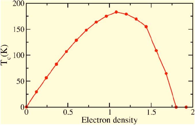
Figure 11:Variation of magnetic T with band filling . Left:(Millis (Chattopadhyay & Millis (2001))) in the limit, for different values of and , . Right: (Brey \cite{dp-brey}) for , , and .
Each of these efforts establish the stability window of ferromagnetic phase, beyond which AF phase was a possibility. The occurrence of non-ferromagnetic phases in spin-fermion problems has been known, and work based on the classical Kondo lattice (Hamada & Shimahara (1995), Agterberg & Yunoki (2000), Alonso et al. (2001), Pradhan & Majumdar (2009)) had revealed that variation in carrier density can lead to a wide variety of magnetically ordered phases.
Figure 12:Schematic of the density of states in (a). the ferromagnetic, and (b). the antiferromagnetic ground states.
Motivated by this a one band `double perovskite’ model had been studied in two dimensions (Sanyal & Majumdar (2009)).
The and denote respectively the creation operators on the magnetic B site (say Fe) and the non-magnetic B sites (say Mo) with the ‘on-site’ energies and . denotes the nearest neighbour hopping between the B-B sites. The are classical localized spins on the B site coupled to electronic spins through coupling . Recalling the level scheme of SFMO in Figure 10, the effective level difference between B and B sites will be . One assumes limit, keeping finite. The parameter space for the problem includes the level difference , electron density , and and the temperature . A schematic of the level scheme and the generic density of states (DOS) in the ferromagnetic and antiferromagnetic case is shown in Figure 12.
In the two dimensional model Sanyal et al (Sanyal & Majumdar (2009)) confirmed the existence of antiferromagnetic (AF) metallic, albeit collinear, phases. The magnetic phases are shown in Figure 13. Ab initio calculations (Sanyal et al. (2009)) in the full 3D situation have since confirmed the possibility of collinear antiferromagnetic metallic phases (Sanyal et al. (2009)).
In three dimensions, however, the magnetic lattice becomes FCC! The frustrated character raises the intriguing possibility of doping driven non collinear antiferromagnetic phases. Part of this thesis will explore this issue in detail.
Figure 13:Left: The magnetic phase diagram of two dimensional model of ordered double perovskite, in electron density and level difference . Right: The snapshot of the magnetic phases, ferromagnet (F), A-type and G-type antiferromagnet.
5Frustrated Mott systems
The Mott metal-insulator transition (MIT), and the proximity to a Mott insulator in doped systems, are crucial issues in correlated electron systems (Mott (1990), Georges et al. (1996), Imada et al. (1998), Dagotto (1994)). Correlated electronic systems involve strong short-range repulsion. At integer filling, the primary effect of correlation is the emergence of an insulating state where band theory predicts a metal. The nature of this insulating state is also different from the band insulator and involves non trivial magnetic correlations.
5.1General introduction
Understanding the transition from a metal to the Mott insulator, and the effect of doping the Mott state, are classic problems in quantum many-body physics. A minimal description is provided by the single band Hubbard model.
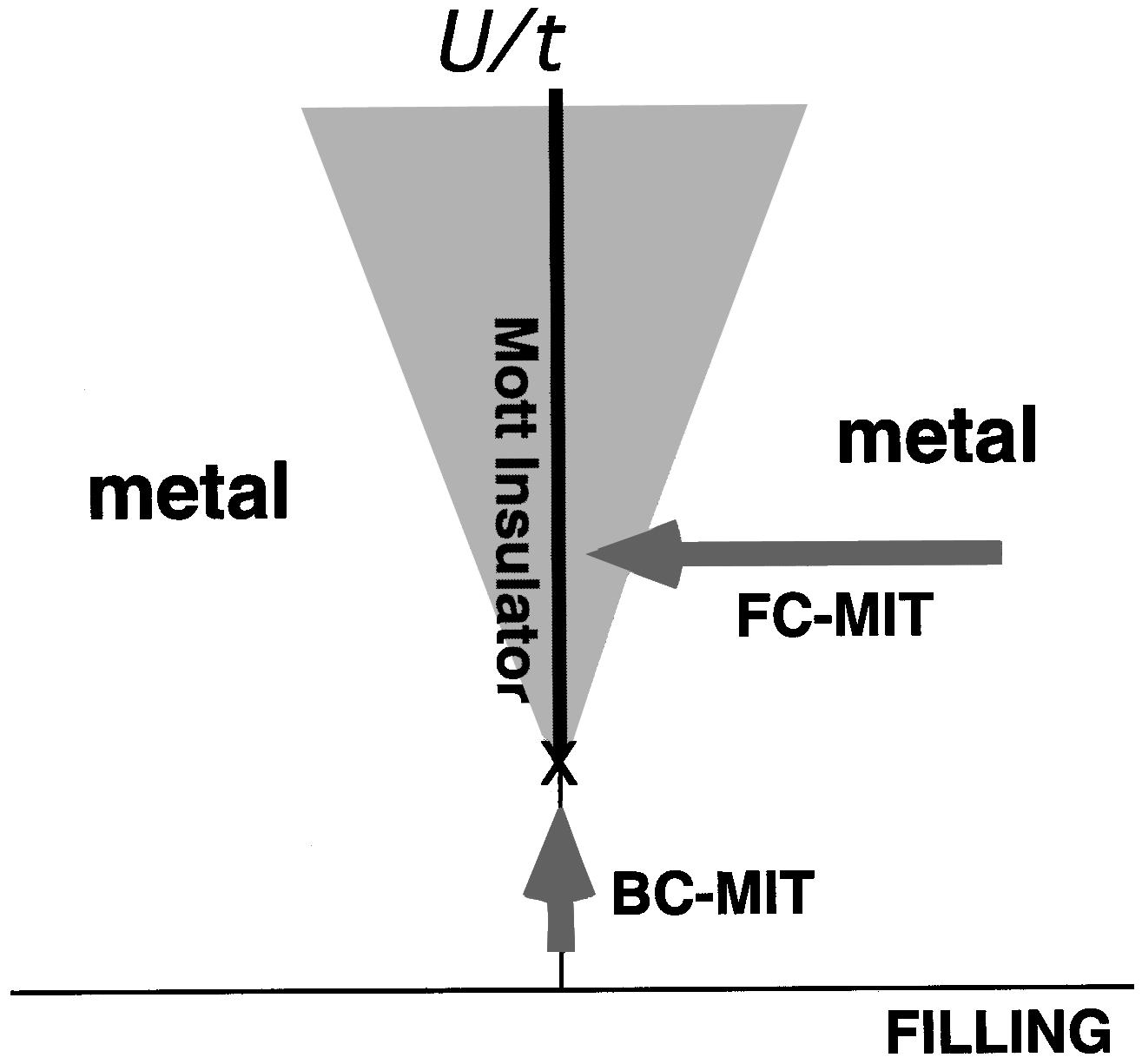
Figure 14:Schematic of the Mott metal insulator transition, showing the filling controlled (FC) transition and the bandwidth controlled (BC) transition. We will focus on the BC scenario in this chapter.
The first term (say ) denotes the kinetic energy involving the hopping amplitudes , usually restricted to nearest neighbours. A given lattice and choices of defines the density of states and bandwidth of the non-interacting systems. The second term, , in equation ((6)) represents the interaction between electrons on the same site. Whether the model has a metallic or insulating ground state depends on the relative strength of interaction and the electron density. A metal-insulator transition (MIT) can be caused, see Figure 14, either by (a) filling control: varying the electron density towards in a large system, or (b) bandwidth control: increasing staying at . In the present thesis we will explore only the bandwidth controlled transition.
While it is large that is ultimately responsible for the Mott phase, the detailed behaviour of the system depends crucially on the symmetry of the underlying lattice, and the hopping parameters . This happens because weak coupling magnetic instabilities depend on nesting features in the Fermi surface, and the magnetism in the Mott phase depends on the lattice geometry. We set down simple features of a few tight binding systems to address the weak coupling physics.
Square lattice with nearest neighbour hopping ()
Square lattice with nearest () and next nearest hopping ()
Triangular lattice, with anisotropic hoppings ()
Figure 15:Schematics of the density of states (upper panel) and electron hoppings (lower panel) for: (a) square lattice with nearest neighbour hopping , (b) square lattice with next nearest neighbour hopping too, and (c) triangular lattice with hoppings , . The Fermi level at half filling is set to .
Figure 15 shows the schematics of hopping amplitudes and and corresponding density of states (DOS) for the above three cases. Their dispersion relations and bandwidth are listed in table below. in Table 2.
Table 2:Dispersion relations of typical 2D lattices.
| Lattice | Hopping | Dispersion | Bandwidth |
|---|---|---|---|
| Square lattice with nearest neighbour hopping | 8 | ||
| Square lattice with next nearest neighbour hopping | 12 () | ||
| Anisotropic triangular lattice | 9 () |
Certain features of the DOS are noteworthy. All the systems (a)-(c) have a logarithmic singularity in DOS. Case (a) has particle-hole symmetry, absent in the other two. The location of the singularity, in terms of band filling, also differs between the three cases. We will see in the chapter Mott transition on the anisotropic triangular lattice, that large DOS near Fermi level results in stronger features in the Linhard susceptibility, which in turn triggers magnetic/charge instabilities in the presence of interactions.
To highlight the basic energy balance involved in the Mott transition we consider the following. The ground state of this tight binding system is the Fermi sea
This by definition is uncorrelated, i.e., occupation of -spin electron on a given site is independent of the occupation of -spin electron on the same site. This means the has a lot of charge fluctuations and double occupancy. The expectation value of the interaction term in the Fermi sea can be calculated as
being the number of lattice sites. The tight binding energy is just the sum of eigenvalues in the occupied part of the band, upto half filling. Assuming just nearest hopping , we have , where is just a number, we have
where, is a number of order 1, which depends on the lattice geometry. The total energy per site, in the uncorrelated ground state is thus
Now consider the state which represents a one electron localized at every site, as would be appropriate deep in the Mott phase. The energy of this state is simply . If we consider only the two limiting cases, and the energies become equal at a .
In reality, the metal suppresses double occupancy with increasing , so it competes better with the localised state. This tends to push higher, as observed in DMFT estimates. Intersite magnetic correlations, on the other hand, stabilise the insulator and tend to reduce below DMFT estimates. So, while the argument for a Mott state at large is quite general, the actual MIT and associated magnetic correlations are very lattice specific.
On a bipartite lattice the Mott transition is well understood in terms of magnetism and transport but the presence of triangular or tetrahedral motifs in the lattice brings in geometric frustration (Ong & Cava (2005), Balents (2010)). This disfavours long range order, and promotes complex electronic states with non-collinear, or incommensurate magnetic character. Their nature, and impact on the MIT, remain an outstanding problem. Such effects have seen some exploration in two dimensions, but hardly any in three dimensions. Below we briefly discuss some key experiments and existing theory in both these cases.
5.2Two dimensional systems
Experiments
In two dimensions, a class of organic compounds provide a concrete testing ground for studying the effects of frustration on the metal-insulator transition (Kanoda & Kato (2011), Powell & McKenzie (2011)). These organics are quasi two dimensional (2D) materials, with molecular formula (BEDT-TTF)X, where -(BEDT-TTF) (also known as -ET) is an organosulfer molecule (Figure 16), and ‘X’ is a halide like anion. The structural information is shown in Figure 17 where (a) shows that the crystal consists of alternating layers of the BEDT-TTF, and the same of halide X ions. In (b) we see the top view of the single layer consisting only of BEDT molecules, which are dimerized, so that the actual ‘intra-dimer’ distances are small compared to ‘inter-dimer’ distance. X being halide, each dimer has deficiency of electron, or a ‘hole’ carrier. If we imagine the dimer as a single ‘site’, then this structure lies on a triangular lattice (Figure 17(c)).
Figure 16:Molecular structure of BEDT-TTF.
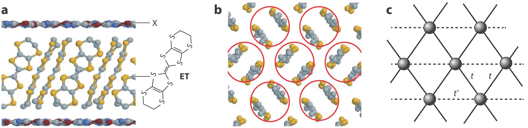
Figure 17:Molecular structure of BEDT-TTF. Right: The crystal structure of the BEDT compounds: (a) in plane view, (b) top view are shown. Assuming each dimer as a ‘site’ they lie on (c) a triangular lattice with anisotropic hoppings ,.
From ab initio calculations, the dimer site is known to be correlated, as the large lattice spacing, , leads to a low bandwidth, enhancing electron correlation effects. The inter-dimer hoppings are anisotropic in general, with one of the three nearest neighbour differing from other two (Kandpal & others (2009)). If we ignore the weak inter-layer coupling the low energy physics can be described by the single band Hubbard model in two dimensions on the anisotropic triangular lattice (Kandpal & others (2009), Shimizu et al. (2011)).
In table Grid a material phase diagram is shown, constructed via ab initio methods (Shimizu et al. (2011)) in which compounds are placed in plane. The parameters are estimated with extended Huckel (EH) and density functional theory (DFT) calculations. A large number of these comounds are close to Mott transition, i.e., can be metalized with moderate pressure. To give a few examples, materials like Cl (Limelette & others (2003)) and CN (Kanoda & others (2011)), which are Mott insulators, undergo an insulator-metal transition (IMT) on hydrostatic pressure of order 20 Mpa. -ClBr shows an IMT as increases above (Yasin & others (2011)).
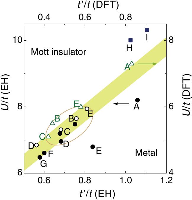
Open circle: Extended Huckel (EH) calculations (120K), Closed circle: EH calculations (290K), Triangle: DFT calculations (taken from Shimizu Shimizu et al. (2011))
| X | |
|---|---|
| A | Cu(CN) |
| B | Cu[N(CN)]Cl |
| C | Cu[N(CN)]Br |
| D | Cu(CN)[N(CN)] |
| E | Cu(NCS) |
| F | Ag(CN)HO |
| G | I |
| H | k-(ET)HgBr |
| I | k-(ET)HgCl |
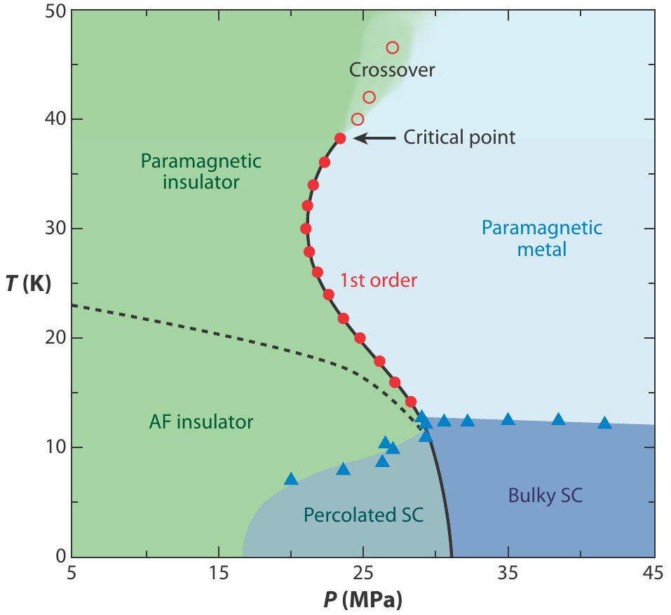
Table 3 shows the experimental ‘pressure-temperature’ phase diagram of the -Cl with pressure and chemical doping, where the MIT boundary is estimated from conductivity measurements. The salient points about the experiments are:
Table 3:Top: The experimental phase diagram with pressure, and doping. Bottom: Corresponding transport measurement as function of temperature. In the second figure, the data from top to bottom are for =0.2,0.4,0.7,0.8,0.85,0.9 and, the absolute values of resistivity are multiplied by and 105 respectively.
 | 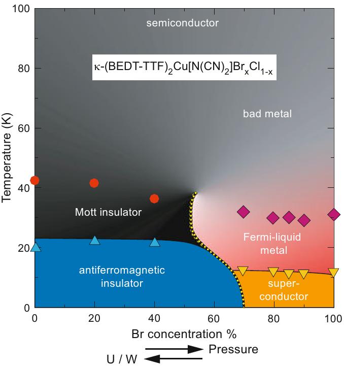 |
|---|---|
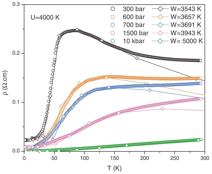 | 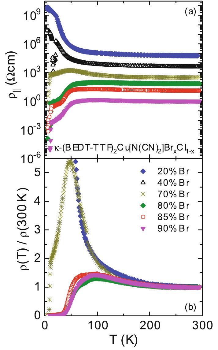 |
The metallic state is very incoherent above K, with mcm (Yasin & others (2011)).
The optical conductivity (Merino & others (2008), Dumm & others (2009)) shows transfer of spectral weight from high frequency, , towards zero frequency and has non Drude character over a pressure window.
The MIT boundary is non-monotonic, i.e, there is reentrance of insulating phase at higher temperature (Dumm & others (2009), Kanoda & others (2011)). See Table 3 top row.
NMR experiments suggests the presence of a pseudogap (PG) (Powell et al. (2009)) in the single particle density of states near the MIT.
The NMR also provides some insight into the magnetic correlations in the material (Powell et al. (2009), Kawamoto et al. (1995), Miyagawa et al. (1995), Shimizu et al. (2003)).
The information about the detailed magnetic state is limited. In Figure 18, (a) shows the magnetic susceptibility at ambient pressure for -CN, and -Cl (b) H-NMR spectra of single crystals of the same. Fitting the susceptibilities of these two to Heisenberg model yields exchanges =240K and 250K. The splitting of the lineshapes of the NMR spectra with lowering temperature indicates the onset of magnetic ordering, which is seen at rather low temperature in -Cl compared to exchange , however the exact nature of magnetic order is not known. On the other hand, for -CN no change is observed down to despite of rather large exchange , suggesting the suppression of long range order because of (greater) frustration.
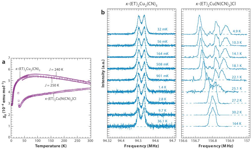
Figure 18:(a) Temperature dependence of the spin susceptibility for -CN, and -Cl. (b) H-NMR spectra for single crystals of -CN, and -Cl under magnetic field applied perpendicular to dimer layer. (Taken from Kanoda & others (2011))
These unusual magnetic states would result in unique transport, optical, and spectral features. Our aim is to uncover the possible magnetic ground state on the frustrated structure and examine the impact of the finite temperature magnetic fluctuations on electronic spectra and transport.
Theoretical background
The single band Hubbard model is the starting point for approaching Mott physics. On the triangular lattice, specifically, there have been several studies (Morita et al. (2002), Watanabe et al. (2008), Inaba et al. (2009), Yoshioka et al. (2009), Tocchio et al. (2009), Limelette & others (2003), Aryanpour et al. (2006), Galanakis et al. (2009), Parcollet et al. (2004), Ohashi et al. (2008), Liebsch et al. (2009), Sato et al. (2012), Sahebsara & Senechal (2008), Yang et al. (2010)) to model organic physics. We quickly review these.
Table 4:Comparison of available many body methods to capture the Mott transition in the 2D triangular lattice. The left most column lists the indicators that we may wish to access to understand the system.
| Method | VMC Tocchio et al. (2009), Tocchio et al. (2013) | ED Koretsune et al. (2007), Clay et al. (2008) | PIRG Imada & Kashima (2000) | VCPT Sahebsara & Senechal (2008), Sahebsara & Senechal (2006) | DMFT Limelette & others (2003), Aryanpour et al. (2006), Galanakis et al. (2009) | CDMFT Parcollet et al. (2004), Ohashi et al. (2008), Liebsch et al. (2009), Sato et al. (2012) |
|---|---|---|---|---|---|---|
| Ground state | Yes | Yes | Yes | Yes | Not yet | Not yet |
| Finite | No | No | No | No | Yes | Yes |
| Density of states | No | Yes | No | No | Yes | Yes |
| Transport/Optics | No | No | No | No | Yes | No* |
| Spatial correlations | Yes | No | No | No | No | limited |
Ground state methods
Variational Monte Carlo (VMC) minimises the energy by optimising the parameters in a variational wavefunction. The minimization of the energy is done via Monte Carlo sampling. This is a real space approach, limited however to small lattice sizes . The reliability of these calculations crucially depend on the quality of trial wave functions. Luca et al (Tocchio et al. (2009)) employed the VMC scheme optimizing two sets of wave functions derived from (a) a mean field Hamiltonian with AF correlations, and (b) BCS Hamiltonian. They concluded that for the MIT occurs at , and the insulating phase is a spin-liquid. Very recently (Tocchio et al. (2013)) they have improved the variational set by taking spiral states. This results in qualitative change in the phase diagram, where at moderate insulating the spin liquid was replaced by spiral antiferromagnets.
Exact diagonalization (ED) As the name suggest, involves numerical diagonalization of the many-body Hamiltonian, using Lanczos algorithm for large sparse matrices. The only limitation is that only lattices with a few sites (of order 16) can be studied. Clay et al(Clay et al. (2008)) studied the Hubbard model at half filling, for all values on a size, and established a phase diagram. They studied the nature of the states and concluded that the model does not exhibit superconducting state.
Path integral renormalization group (PIRG) method (Imada et al Imada & Kashima (2000)) constructs an optimized ground state wave function as a linear combination within the allowed dimension , of the Hilbert space in a numerically chosen basis . The ground state is projected out after successive renormalization process in the path integral, in a manner in which both the coefficients and the basis is optimized.
Variational cluster perturbation theory (VCPT) divides the lattice into identical clusters of size (say) with the inter-cluster hoppings, and evaluates one particle Green’s function within the cluster numerically with open boundary conditions. The inter-cluster hoppings are treated perturbatively to recover the full Green’s function . Depending on the size , short range correlations can be accessed in the system.(Sahebsara et al Sahebsara & Senechal (2008), Sahebsara & Senechal (2006)).
To have a feel on how some of these method compare when accessing the ground state, we show, in Figure 19 the ground state phase diagram using four different methods. (a) VMC by Luca et al (Tocchio et al. (2009), Tocchio et al. (2013)), (b) ED by Clay et al (Clay et al. (2008)), and (c) VCPT by Sahebsara et al (Sahebsara & Senechal (2008), Sahebsara & Senechal (2006)).
Figure 19:Ground state phase diagram of the Hubbard model on the anisotropic triangular lattice. Notation for the phases is standard, except TRI: 120 ordered insulator, and dSC: wave superconductor.
Access to finite temperature has been usually with dynamical mean field theory(DMFT). It has been the method of choice (Limelette & others (2003), Aryanpour et al. (2006), Galanakis et al. (2009)), mapping the many body lattice problem to a many body local problem, supplemented by a self-consistency condition (Georges & Kotliar (1992)). Some spatial correlations can be included via cluster DMFT (Parcollet et al. (2004), Ohashi et al. (2008), Liebsch et al. (2009), Sato et al. (2012)). Figure 20 shows phase diagram for anisotropic triangular lattice established by (a) Ohashi et al (Ohashi et al. (2008)) for using 4 site cluster based C-DMFT, and by (b) Liebsch et al (Liebsch et al. (2009)) using 3 site cluster. They use the double occupancy to characterize the Mott transition.
Though the method captures the reentrance in MIT, as the Figure 20 shows, the understanding of its origin isn’t present. Besides they present it in a limited window of .
We summarize below the results of the above methods, skipping the detailed discussion for later in chapter Mott transition on the anisotropic triangular lattice. On triangular motif, the results in general depend on the degree of frustration and the specific method, but broadly suggest the following:
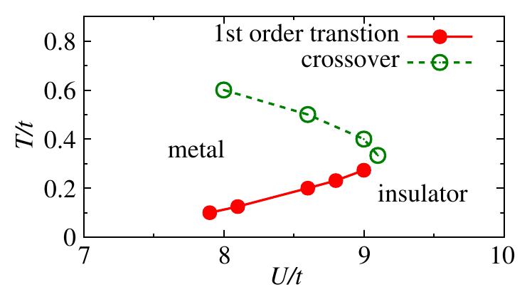
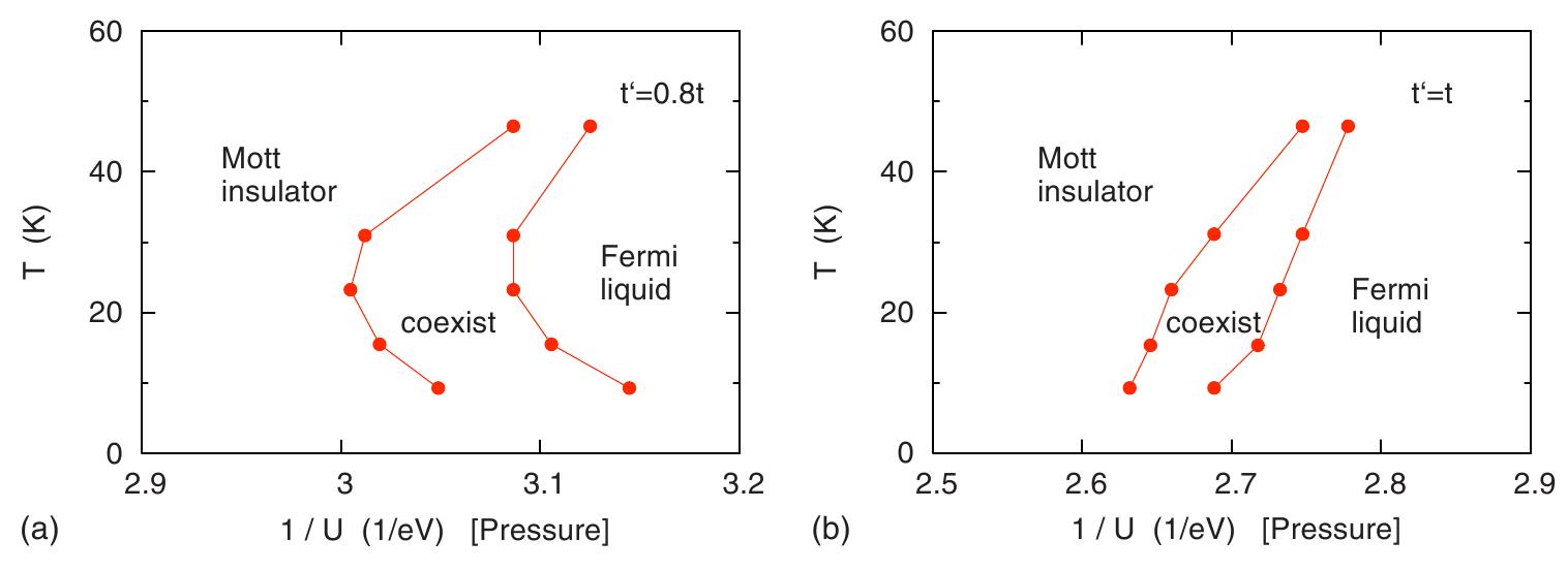
Figure 20:Finite temperature phase diagrams established by C-DMFT. Top: Bottom: (a) and (b)
The ground state is a paramagnetic Fermi liquid at weak coupling, a `spin liquid’ or para-insulator at intermediate coupling, and an antiferromagnetic insulator at large coupling (Morita et al. (2002), Watanabe et al. (2008), Inaba et al. (2009), Yoshioka et al. (2009), Tocchio et al. (2009)).
The qualitative features in optics (Merino & others (2008)) and transport (Limelette & others (2003)) are recovered.
There could be a reentrant insulator-metal-insulator transition with increasing temperature for a certain window of frustration (Ohashi et al. (2008), Liebsch et al. (2009)).
A low temperature superconducting state could emerge (Watanabe et al. (2006), Kyung & Tremblay (2006), Liu et al. (2005)), although Clay et al (Clay et al. (2008)) deny this possibility.
The following are the open issues
Most of the real space techniques are for , except DMFT which ignores spatial fluctuations. CDMFT does capture short range correlations but has not been generalised to handle complex magnetic states (Ohashi et al. (2008)).
There is very limited data on transport (Merino & others (2008), Limelette & others (2003)), obtained mainly via DMFT. These do not capture the effect of magnetic correlations close to the Mott transition.
Similarly, there is no study of the angular anisotropy of the pseudogap and its connection to magnetic correlations close to Mott transition.
We use a real space approach that is complementary to DMFT, handles spatial fluctuations and inhomogeneity well at finite temperature, and can provide a comprehensive answer to these questions.
5.3Three dimensional systems
Three dimensional frustrated systems usually have tetrahedral connections. Examples are FCC and pyrochlore lattice (see Figure 21). Below we review the experimental literature, and theoretical development of these three dimensional frustrated correlated systems.
Figure 21:Up/Left: FCC lattice, where green spheres denote the sites. The nearest neighbours form tetrahedral motif, which is the geometric ingredient for frustration. Down/Right: pyrochlore lattice, seen as FCC lattice with a basis of four site tetrahedra (denoted by black, red, green and blue spheres). The nearest neighbours are connected by blue lines within the basis, and red lines among neighbouring basis.
Experiments
While there has been intense exploration of frustration effects in two dimensions, as we saw in the last section, there is no organized body of work probing the interplay of geometric frustration and Mott physics in three dimensions. The systems with geometric frustration in 3D are realized on (a) the FCC lattice and (b) the pyrochlore lattice. In Figure 21, the lattice structure with nearest neighbour connection is shown for (a) the FCC lattice, which consists of edge sharing tetrahedra, and (b) the pyrochlore lattice, which consists of corner sharing tetrahedra.
There are, however, intriguing experiments on rather disparate systems whose common features do not seem to have been noticed, and no theoretical effort to connect them. The FCC examples include
Cluster compounds (CC) of formula AMX (Pocha & others (2005), Jakob & others (2007), Abd-Elmeguid & others (2004), Phuoc & others (2013)), where A is usually Ga or Ge, M is transition metal and X is S or Se. In these compounds the electronically active units are the ‘cluster’ M, which have one unpaired electron per cluster.
Some alkali fullerides of the form AC (Takenobu et al. (2000), Capone & others (2009), Ganin & others (2010), Ihara et al. (2010)), which have C ions on FCC lattice. CsC (Ganin & others (2010)) for example, is magnetic insulator at ambient pressure, and becomes superconducting under pressure. It exists in two crystalline forms, one in which the anion is FCC, the other in which its BCC. At ambient pressure, the frustrated FCC polymorph has much lower Neel temperature T, compared to the BCC polymorph (T).
The site ‘B’ ordered double insulating perovskites, e.g., SrInReO (Gao & others (2011)). Many of these do not show long range order but spin-glass (Wiebe et al. (2002), Aharen & others (2009), Aharen & others (2010)), or valence bond glass (Vries et al. (2010)) character instead.
The pyrochlore examples include the molybdates RMoO (Gaulin et al. (1992), Gingras et al. (1997), Iguchi et al. (2009)), and iridates EuIrO (Nakatsuji & others (2006), Matsuhira & others (2007), Ueda et al. (2012), Tafti et al. (2012)). Most of these materials are insulators close to a Mott transition. They exhibit complex magnetic order, including a ‘spin frozen’ state, and have unusual Hall response (Machida et al. (2007)) indicative of non coplanar order. They show have unusual temperature dependence in the resistivity - larger in metallic state at high temperature than the insulating state.
Table 5:Summary of experimental results available on three dimensional frustrated compounds potentially close to a Mott transition.
| Compound | GaMSe | AC | ABBO | RMO |
|---|---|---|---|---|
| Structure | FCC (Pocha & others (2005)) | FCC, A15 (Capone & others (2009)) | FCC | Pyrochlore |
| Pressure studies | Hydrostatic | Hydrostatic, doping (Takenobu et al. (2000)) | None | Hydrostatic(Tafti et al. (2012), Iguchi et al. (2009)) |
| Reference state | Mott insulator | Mott insulator | Mott insulator or metal | Mott insulator or metal |
| Measurements | Resistivity, optical conductivity, Susceptibility | NMR (Ihara et al. (2010)) | Susceptibility(Gao & others (2011), Wiebe et al. (2002),Aharen & others (2009), Aharen & others (2010)) | Resistivity (Tafti et al. (2012), Iguchi et al. (2009)), Hall effect (Machida et al. (2007)), Susceptibility (Gingras et al. (1997)) |
| Magnetic state | Glassy (Pocha & others (2005)), Flux(Jakob & others (2007)) | Supercond (FCC), AF (A15) | Spin glass (Gao & others (2011), Wiebe et al. (2002), Aharen & others (2009), Aharen & others (2010)), VBS(Vries et al. (2010)) | Spin glass (Iguchi et al. (2009), Gaulin et al. (1992), Gingras et al. (1997)) |
Let us focus on the FCC cluster compounds which seem amenable to modelling within the single band Hubbard description.
AMX compounds
The crystal structure of the AMX compounds, is shown in Figure 22a. The electronic correlation arise due to the large distance between clusters, , compared to the intra-cluster distances. According to molecular orbital (MO) calculations, the orbitals hybridize to form MOs which consist of three different bonding states (a) a non degenerate level followed by (b) two fold and (c) three fold levels (see Figure 22b). For A=Ga, we have 7 electron per cluster for M=V,Nb,Ta and 11 electrons for M=Mo. In both cases, the occupation of cluster levels corresponds to one unpaired electron per cluster. This is at the heart of the single band Hubbard description.
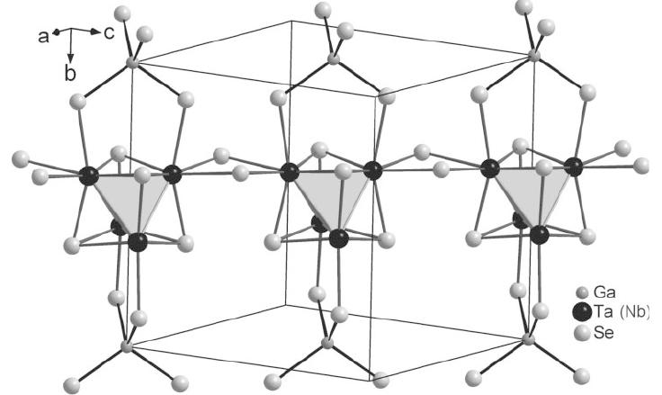
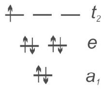
Figure 22:Left: Crystal structure of AMX systems. Right: Molecular orbital scheme for bonding of M clusters for seven electrons per cluster.
Early measurements (Abd-Elmeguid & others (2004)) on GaNbSe and GaTaSe revealed a pressure driven IMT at moderate pressure ().
At ambient pressure the materials are insulating with gaps eV and 0.1eV, respectively.
Increasing pressure (GPa) leads to a phase with large but finite resistivity at T=0, and . This persists over a pressure window beyond which they behave like conventional metals (see Figure 23a).
A very recent optical conductivity measurement on GaTaSe (Figure 23b) indicates that the pressure driven transition involves large transfer of low frequency weight and should be thought of as a Mott transition.
Few magnetic measurements on GaNbSe(Pocha & others (2005)) suggest a large Curie-Weiss constant (K), but difficult to detect, suppressed non-collinear ‘flux’ like order (Jakob & others (2007)).
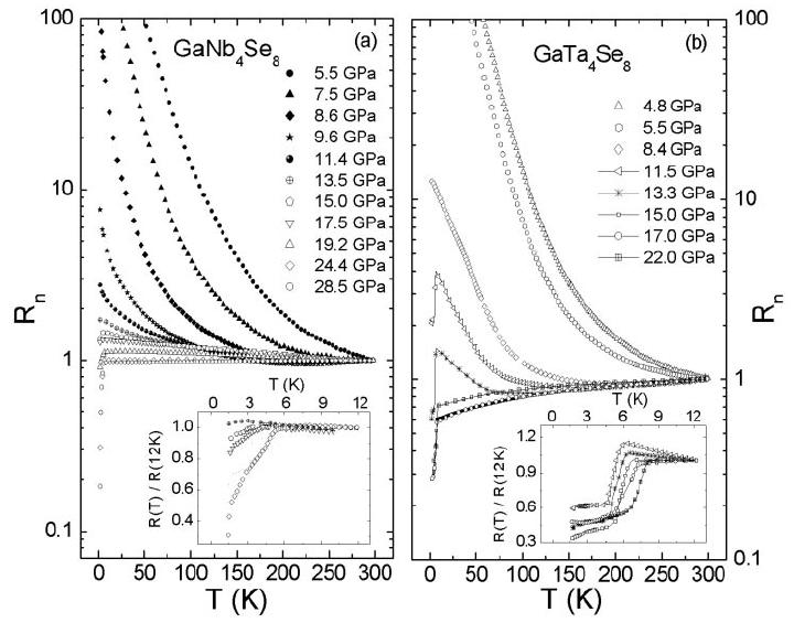
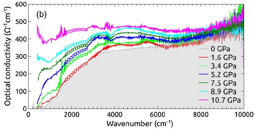
Figure 23:Resistivity (up/left) and the optical conductivity (down/right) in AMX systems.
Theoretical background}
One can understand the pressure driven Mott transition in the cluster compound, in terms of single band Hubbard model defined on the FCC lattice at half filling, where the M clusters are mapped to a correlated site with Hubbard repulsion and nearest neighbour electron hopping . Qn the FCC lattice, surprisingly, there is hardly any theoretical work, except very early attempts using conventional static mean field theory\cite{mf-fcc}. A very recent paper, Phuoc et al(Phuoc & others (2013)), does present a DMFT based phase diagram, but there is no discussion about the nature of spatial fluctuations, which could play a crucial role in the frustrated system.
6Agenda of the thesis
We have briefly reviewed the experimental background and theoretical progress in two situations:
a. double exchange driven magnetism in double perovskites, and
b. pressure driven metallisation of frustrated Mott insulators.
In both cases, the nature of magnetism has been a puzzle due to the frustrated lattice geometry. Establishing the nature of magnetic correlations and possible long range order, driven by electron delocalisation, defines the first task in the problems above.
The nature of the magnetic background affects the electronic spectrum and transport, quantifying this defines the second task. In particular, the metal-insulator transition in the ground state, and a possible pseudogapped phase in the vicinity of the MIT, is one important issue. In addition, thermal fluctuations have a dramatic effect on the low frequency density of states, the angle resolved spectrum, the resistivity, and the optics. Establishing the behaviour of these indicators in our models, and comparing with available experimental data will be the major task.
There is a wealth of data in two dimensions from the organics, and some scattered data in three dimensional frustrated materials close to the Mott transition. We will use a Hubbard-Stratonovich decomposition to construct a ‘lattice field theory’ of electrons coupled to auxiliary moments and try to provide a qualitative overview and a detailed quantitative description of Mott physics in these systems, and compare in detail with available experimental data.
- Wannier, G. . H. (1950). Phys. Rev., 79, 357.
- Kano, K., & Naya, S. (1953). Prog. Theor. Phys., 10, 158.
- Vacks, V., Larkin, A., & Ovchinnikov, Y. (1966). Sov. Phys. JETP, 22, 820.
- Morita, T., Chikyu, T., & Suzuki, M. (1987). J. Phys. A, 19, 1701.
- Morita, T., Chikyu, T., & Suzuki, M. (1987). Prog. Theor. Phys., 78, 1242.
- Azaria, P., Diep, H. T., & Giacomini, H. (1987). Phys. Rev. Lett., 59, 1629.
- Debauche, M., & Diep, H. T. (1992). Phys. Rev. B, 46, 8214.
- Mézard, M., Parisi, G., Sourlas, N., Toulouse, G., & Virasoro, M. (1984). Phys. Rev. Lett., 52, 1156–1159.
- Parisi, G. (1983). Phys. Rev. Lett., 50, 1946.
- Diep, H. T. (2005). Frustrated spin systems. World Scientific.
- Moessner, R., & Chalker, J. T. (1998). Phys. Rev. B, 58, 12049.
- Moessner, R., & Chalker, J. T. (1998). Phys. Rev. Lett., 80, 2929.
- Huse, D. A., & Rutenberg, A. D. (1992). Phys. Rev. B, 45, 7536.
- Chalker, J. T., Holdsworth, P. C. W., & Shender, E. F. (1992). Phys. Rev. Lett., 68, 855.
- Lecheminant, P., Bernu, B., Lhuillier, C., Pierre, L., & Sindzingre, P. (1997). Phys. Rev. B, 56, 2521.