Mott physics and glassiness on the FCC lattice
In the previous chapter we saw how geometrical frustration in the triangular lattice disfavours Neel order and promotes complex non-collinear states. There are several families of compounds based on three dimensional frustrated lattices. The complexity of the these structures has prevented a detailed exploration of Mott physics and the possible magnetic phases.
1Background
Unlike in two dimensions (2D), there is no organized body of work probing the interplay of geometric frustration and Mott physics in three dimensions (3D). In 3D there are intriguing experimental results on disparate systems (Pocha & others (2005), Jakob & others (2007), Abd-Elmeguid & others (2004), Phuoc & others (2013), Takenobu et al. (2000), Capone & others (2009), Ganin & others (2010), Ihara et al. (2010), Wiebe et al. (2002), Aharen & others (2009), Aharen & others (2010), Vries et al. (2010), Gao & others (2011), Gaulin et al. (1992), Gingras et al. (1997), Iguchi et al. (2009), Nakatsuji & others (2006), Matsuhira & others (2007), Machida et al. (2007), Ueda et al. (2012), Tafti et al. (2012)), whose common features do not seem to have been noticed. The 3D frustrated Mott systems are realized on face centered cubic (FCC) and pyrochlore lattices. They both involve connected tetrahedra, disallowing Neel order in the insulating phase. The FCC examples include the Ga cluster compounds (Pocha & others (2005), Jakob & others (2007), Abd-Elmeguid & others (2004), Phuoc & others (2013)), alkali fullerides, AC (Takenobu et al. (2000), Capone & others (2009), Ganin & others (2010), Ihara et al. (2010)), and the double perovskites (Wiebe et al. (2002), Aharen & others (2009), Aharen & others (2010), Vries et al. (2010), Gao & others (2011)). The pyrochlore examples include the rare earth molybdates (Gaulin et al. (1992), Gingras et al. (1997), Iguchi et al. (2009)) and iridates (Nakatsuji & others (2006), Matsuhira & others (2007), Machida et al. (2007), Ueda et al. (2012), Tafti et al. (2012)). Most of these materials, at ambient pressure (undefined (n.d.)), are insulators close to a Mott insulator-metal transition (IMT). Despite the wide chemical variety, several striking features seem to be common:
Magnetic state: The Mott phase often has no long range magnetic order down to the lowest temperature, only short range antiferromagnetic correlations and sometimes a hint of ‘spin freezing’ (Gao & others (2011), Aharen & others (2009), Vries et al. (2010), Aharen & others (2010), Gaulin et al. (1992), Gingras et al. (1997)). However, many of these systems have large Weiss constant (see Table 1), suggesting strong antiferromagnetic exchange. This indicates a high degree of frustration in such systems.
Unusual metal: The Mott insulator can be driven metallic by applying pressure. The resulting state is a ‘non Fermi liquid’ - with anomalously large low temperature resistivity and a negative temperature coefficient (Abd-Elmeguid & others (2004), Iguchi et al. (2009), Ueda et al. (2012), Tafti et al. (2012)). At high pressure ‘normal’ metallic behaviour is observed.
Anomalous Hall: Several of these systems have non-coplanar antiferromagnetic correlation. For example GaNbSe (Jakob & others (2007)) exhibits long range non-coplanar antiferromagnetic order with . This can lead to anomalous Hall response, as already observed in the pyrochlore iridate PrIrO(Machida et al. (2007)).
Spectral weight transfer: The optical conductivity(Phuoc & others (2013), Ueda et al. (2012)) indicates that the insulator to metal transition involves transfer of spectral weight over a wide frequency window.
Superconductivity: Some of these systems, e.g, the cluster compounds (Abd-Elmeguid & others (2004)) and the alkali fullerides (Takenobu et al. (2000), Capone & others (2009), Ganin & others (2010), Ihara et al. (2010)), show superconductivity at low temperature.
Table 1:Curie constants of some of the FCC and pyrochlore compounds.
| Compound | Structure | () | Reference |
|---|---|---|---|
| GaNbSe | FCC | 300 | Pocha & others (2005), Jakob & others (2007) |
| CsC | FCC | 105 | Ganin & others (2010) |
| BaYRuO | FCC | 571 | Aharen & others (2009) |
| SrInReO | FCC | 182 | Gao & others (2011) |
| BaYMoO | FCC | 160 | Vries et al. (2010) |
| YMoO | Pyrochlore | 200 | Gingras et al. (1997) |
The first three features are direct consequences of frustration which promotes non-coplanarity and short range correlation, in contrast to collinear long range order. The last two are more generic to Mott physics. We will show that the single band Hubbard model on the FCC lattice helps us understand the connection between magnetism and transport in a subset of these materials (Abd-Elmeguid & others (2004), Phuoc & others (2013)). Based on our solution of the Mott problem on the FCC lattice we establish the following.
In the ground state, increasing interaction leads, successively, to transition from a paramagnetic metal (PM) to a spin glass metal (SGM), a spin glass ‘insulator’ (SGI), and then an antiferromagnetic insulator (AFI). The spin glass arises without the presence of any extrinsic disorder, consistent with several frustrated materials. The AFI has flux like order (defined later) at weaker coupling, and ‘C type’ order in the very strong coupling Heisenberg limit.
The scales in the ordered phase, as well as the notional glass transition temperature , are a tiny fraction, a few percent, of the hopping scale due to the frustration.
While the AFI phase has a clear gap and divergent resistivity as temperature , the spin glass insulator has a pseudogap in the density of states, non Drude optical response in the optical conductivity, and large but finite resistivity at with with negative temperature coefficient ().
The results above, although obtained for the FCC lattice, have much in common with observations on the pyrochlores.
We have found little theoretical work on the magnetic phases or the Mott transition in the FCC lattice. A very early calculation explored a restricted set of mean field states (Grensing et al. (1978)) but, in contrast to 2D, there does not seem to be any cluster dynamical mean field theory (C-DMFT) result handling the combination of correlation and frustration.
As before we study the following model at half filling:
The denote nearest neighbours on the FCC lattice. We set as the reference energy scale. controls the electron density, which we maintain at half filling . is the Hubbard repulsion. Using the Hubbard-Stratonovich (HS) approach used in the last chapter, we get the following effective Hamiltonian which describes electrons moving in the spatially fluctuating background of classical fields (where )
We can write this as sum of electronic and classical part , where . The configurations follow the distribution
Retaining the spatial fluctuations of allows us to estimate scales, and access the crucial thermal effects on transport. Within the static HS approximation and define a coupled fermion-local moment problem. This is similar to the ‘double exchange’ problem, with the crucial difference that the moments are self generated (and drive the Mott transition) and are not fixed in size.
As before we use a Monte Carlo technique, now on lattices upto in size, with clusters of size . For characterising the magnetic state we calculate the thermally averaged structure factor at each temperature. The onset of rapid growth in at some , say, with lowering , indicates a magnetic transition. Electronic properties like density of states, optical conductivity etc, are calculated by diagonalizing on the full lattice for equilibrium configurations. Since the MC ground state can be affected by annealing protocol, wherever possible we have tested it against variational choices of .
In the next Section 2, we discuss the ground state. In Section 3, we take up the finite temperature physics in detail, including the behaviour of the auxiliary fields, the density of states across the Mott transition, and transport and optical properties. This is followed by a section comparing our results with recent measurements on the FCC based Ga cluster compounds. We then conclude the chapter.
2Ground state
At , the Monte-Carlo based sampling becomes the minimization process
Please note that need not be periodic. We observe the following with growing in the ground state.
At low the minimization leads to a state with vanishing moments . This holds for .
There is a weakly discontinuous transition to a state with non-zero at . For , where , the ground state involves finite , with a finite width distribution (see later) but no long range order. The system behaves like a spin glass (SG) with short range ‘flux like’ correlations.
Beyond the ground state has long range flux like order till , beyond which the virtual hopping generated exchange is effectively nearest neighbour and we obtain ‘C type’ order, as expected (Gvozdikova & Zhitomirsky (2005)) for the AF Heisenberg model on the FCC lattice.
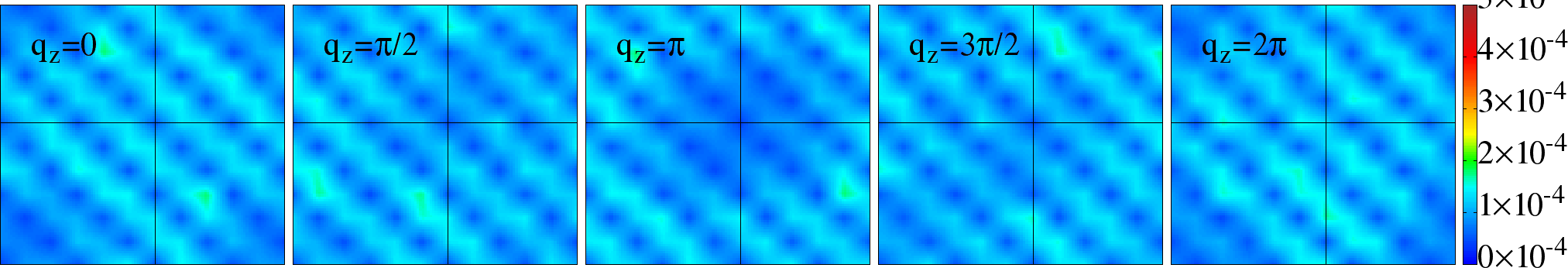
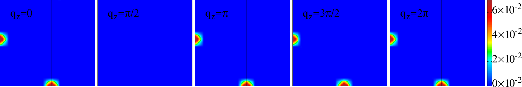
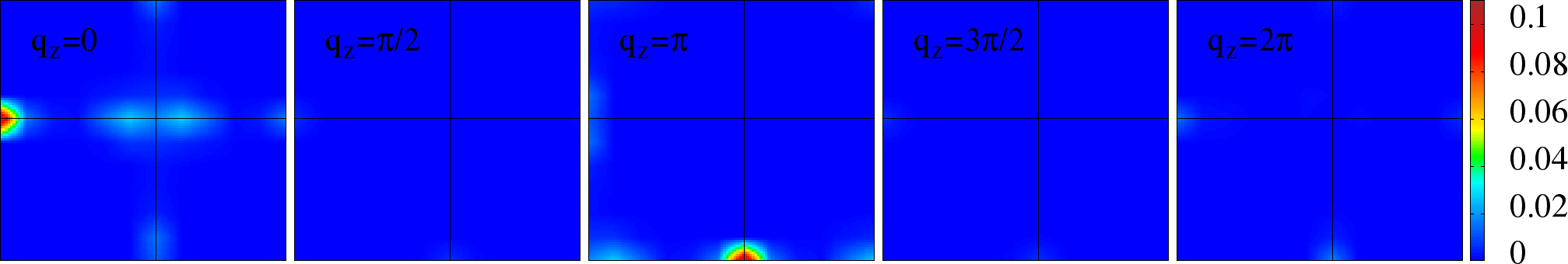
Figure 1:Two dimensional cross sections of the structure factor data at low temperature, for: top row: in the spin-glass region, middle row: for flux like order, and bottom: for C type order. Each row has color plots of in the , with selected .
Figure 1 shows the structure factor that emerges from annealing the system to low temperature at three values of . For , top row, the pattern does not show any signature of long range order but does have moments as Figure 2 reveals. At the structure factor (middle row) shows flux like order, with a fairly large moment, while at the magnetic order is C type.
At the density of states, Figure 2 right panel, is almost featureless. The system is a metal, to be cross checked later via actual resistivity calculation. At the two larger values of there is a clear gap in the spectrum and the system is an insulator. The DOS plots reveal that between the simple metal and the hard gap insulator there is a pseudogap phase. That turns out to have insulating resistivity as we will see later.
We now move to a quick analysis of the weak coupling and strong coupling phases using the same tools that we used for the triangular lattice.
Figure 2:Low temperature behaviour: The left panel shows the distribution of the magnitude of the moments. Right: the electronic DOS in the corresponding backgrounds. Notice the broad distribution with a small mean that arises at intermediate , and the much sharper (ideally function) at larger values of . The DOS shows a pseudogap in the glassy phase.
2.1Weak Coupling
In the 2D triangular lattice we could get some insight about the low magnetic state by examining the RPA susceptibility based on . In that problem the peak location of provided a hint about possible magnetic order.
We tried the same calculation in the FCC case but visualisation of the data is now more difficult. Instead of attempting to show a 3D plot of we have shown cross sections of in the plane for various choices of . The two rows in Figure 3 show data for the FCC (top row) and the simple cubic lattice (bottom row). The simple cubic case has a clear peak at while the the FCC result shows a featureless with the value ranging from as one moves over the Brillouin zone.
![2D cross sections of tight binding susceptibility \chi_{0}({\bf q}) for (Top) the FCC lattice and (Bottom) the simple cubic lattice. The figures are in q_x,q_y planes, for selected q_z values shown in the figures in the range [0, 2\pi].](/thesis/build/chi-fcc-2d-dc5b14616767d0bc334e721d2c604ae1.png)
![2D cross sections of tight binding susceptibility \chi_{0}({\bf q}) for (Top) the FCC lattice and (Bottom) the simple cubic lattice. The figures are in q_x,q_y planes, for selected q_z values shown in the figures in the range [0, 2\pi].](/thesis/build/chi-sc-2d-74c3ab5fec82b7914e893306e89024d9.png)
Figure 3:2D cross sections of tight binding susceptibility for (Top) the FCC lattice and (Bottom) the simple cubic lattice. The figures are in planes, for selected values shown in the figures in the range [0, ].
Remembering that at weak coupling we can use an effective model of the form
to locate the instability, the result suggests that a simple ordered state may not be the optimal solution. What we discover instead is that for beyond a threshold the system generates a small moment which freezes into a glassy state (with short range flux like correlations), see Figure 1a.
The moment is not large enough, near , to kill the metallic state, but it generates a residual resistivity. With growing the density of states shows a pseudogap, and increasingly larger resistivity and for the spectrum shows a hard gap. Within our resolution that is also where the moments order into a long range flux like pattern.
2.2Strong coupling
At very strong coupling, deep into the Mott phase, the leading order virtual hopping process generates the effective model
For nearest neighbour this is the classical antiferromagnetic Heisenberg model on the FCC lattice. Had we retained the quantum dynamics of the we would have obtained the quantum Heisenberg model.
The classical model has been well studied (Gvozdikova & Zhitomirsky (2005), Ader (2001), Ader (2002), Sousa & Plascak (2008)), and extensive Monte Carlo results suggest the occurence of ‘C type’ order, see Figure 4, right. The nearest neighbour model has large degeneracy in \cite{heis-fcc1}, however the thermal effects, and a small next nearest neighbour coupling, select collinear configuration.
Our results in the large limit confirm this, and also generate the correct scale . At weaker coupling but still in the Mott state we obtain a flux like configuration, Figure 4 left, as the ground state, probably because longer range hopping processes generate multispin couplings favouring non coplanar order.
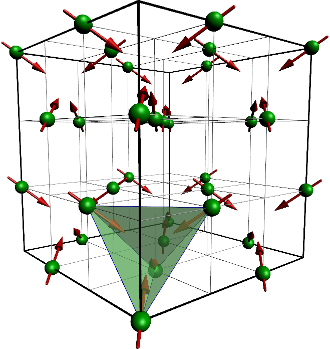 | 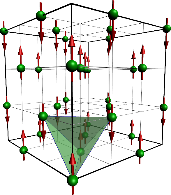 |
|---|
Figure 4:The configuration in the flux state (left) and the C-type state (right). The FCC lattice points are shown by green spheres, and the fields by red arrows.
3Finite temperature properties
3.1Phase diagram
The ground state, as we have discussed, involves the sequence PM SGM SGI AFI (flux and then C type) with increasing interaction. The main issues of interest in characterising the finite phases are:
The , and glass transition scale .
The single particle DOS in terms of gap or pseudogap.
The transport character, {\it i.e}, or .
The nature of magnetic order and is established from the structure factor peak. In the absence of a ordering peak in the structure factor the ‘relaxation time’ yields an estimate of freezing temperature. These are discussed in the next section.
Figure 5:The phase diagram. In ground state, upon increasing , the system goes from PM (with no local moments) to successively, spin glass SGM, SGI (with disordered local moments), then to ordered AFI. At finite temperature the system also has a paramagnetic (Mott) insulating (PI) phase. The magnetic transition temperature , and the spin glass freezing temperature (see text), are indicated. We show the extrapolation of the asymptote, that describes the transition, to highlight the large deviation from the short range Heisenberg result. The PG region involves a pseudogap in the density of states.
Overall, the phase diagram Figure 5 indicates that deep in the Mott phase follows the Heisenberg result, but is already significantly different by the time . For the size of the local moment itself diminishes rapidly, due to increase in itinerancy, and the falls sharply.
Below we have a glassy phase where, the field seem to freeze at low temperature. We make a crude estimate of the ‘freezing temperature’ from the MC based local relaxation time (Binder & Young (1986)), (discussed in the next section Section 3.2). If the system undergoes an ordering transition, on lowering , there is a rapid growth in accompanied by a growth in the structure factor at the 's associated with long range order (LRO).
For a glass transition, one observes similar growth in , without any signatures in . For we observe LRO as well as a rapid increase in at a single temperature . For the window , however, rises, at a temperature we call , without associated LRO. We have also `heated’ the system up from and discovered that any assumed ordered state is quickly destabilized, while the moments themselves survive. varies in the manner shown in Figure 5, vanishing for where there are no local moments. The freezing scale monotonically increases from and matches the of the flux phase at .
The large regime is obviously gapped due to the presence of large moments, which prevent double occupancy, and the small regime has a density of states that is weakly renormalised with respect to the band result. At intermediate , where the moments are small {\bf and} disordered the electron spectrum only shows a suppression of weight at the Fermi level and not a full gap. This window is marked as PG in the phase diagram. Any mean field treatment of the magnetic problem would have yielded a ‘band structure’ for the electrons. The novelty in the present case, with respect to the triangular lattice situation, is that the PG window survives down to due to the presence of disordered local moments. The DOS will be shown in detail in a later subsection.
Figure 6: dependence of the distribution at (a) =0.03 showing weak , and broad distribution around it in the correlated metal to, progressively stronger , and sharper distribution in the AFI with increasing . (b) The same for =0.2, where all the have progressively become broader and with higher , as compared to those in (a).
The ‘metallic’ and ‘insulating’ characterisation is done by examining the temperature derivative . We will see the detailed resistivity later. For the moment notice that in addition to the obvious crossover from insulating to metallic behaviour with decreasing interaction we can have an I-M crossover (in a narrow window) by increasing temperature as well.
3.2Auxiliary fields
We first consider the magnitude distribution of the auxiliary field. In Figure 6 and Figure 7 we have shown the evolution of of the auxiliary fields . Figure 6(a) and Figure 6(b) show the dependence, respectively, at low temperature, , and high temperature, . Figure 7(a)-(c) shows the temperature evolution at three representative values of , (a) when the system is a SG metal, (b) =, and (c) = when in SG insulator. The trends in the broadening of the distribution with increasing temperature and interaction strength are qualitatively same as in two dimensions.
We calculate the structure factor
for the angular spatial correlation, and the average relaxation time to get the correlation in the ‘MC’ time.
Figure 7:Temperature dependence of the distribution at three fixed in the SG window. (a) , (b) = and (c) =.
In Figure 8 we have shown the temperature dependence of the structure factor and the relaxation time. The onset of rapid growth in at some , defines onset of long range order, while the particular sets of s define the precise nature of the order. The onset of rapid growth in , shows the tendency of ‘freezing’ of the auxiliary fields in the `MC’ time. The freezing temperatures, and the magnetic transition temperature are marked in the figure as onset of growing and respectively. Beyond , till , we get a ‘flux’, phase, after which we get the ‘C type’ antiferromagnetic phase, which have the growing set of mentioned in the table \ref{tabqfcc}. The nature of these states is shown in Figure 4.
Table 2:The s for the flux and C type.
| Phase | |
|---|---|
| Flux | (,,0),(0,0,),(,0,),(0,,0),(0,,),(,0,0) |
| C type | (,,0),(0,0,) |
Figure 8:Temperature dependence of , and at . (a) where, shows no growth, down to for any , while starts growing around . (b)-(d) for respectively, where and both grow at the same temperature ().
3.3Density of states
While in the insulating phase () the system would have a gapped density of states (DOS), and in the metallic () case is likely to have a featureless DOS, the glassy window in between may have unusual spectral features. Figure 9.(a)-(b) shows the DOS for varying at and , respectively. For lack of space in the figure, the colour codes for are marked in panel (b) only. In panel (a), for the DOS is featureless, but for it displays a pseudogap (PG), and for higher there is a clear gap. The large phase is magnetically ordered at this temperature. At the higher temperature in panel (b), where there is no trace of magnetic order, the PG feature extends over a much larger window. The weaker ‘metals’ in (b) have a deeper PG compared to panel (a), while the weak gap insulators now have a PG feature rather than a hard gap. Panel (b) essentially illustrates the paramagnetic Mott transition on the FCC lattice.
Figure 9: dependence of density of states at (a) =0.03 showing the crossover from correlated metal to AFI through a wide pseudogap window, and (b) =0.2, where the crossover is between the PM and a PI through a much wider pseudogap window.
Figure 10:Temperature dependence of density of states at three fixed in the SG window. See the thermally induced PG at weak (a), the presence of the PG at itself for (b) = and (c) =.
Panels Figure 10.(a)-(c) show the dependence of the DOS for three typical in the glassy window, where the ground state has frozen local moments. They all share the feature of thermally induced loss of low frequency weight which shows up at . There is markedly less change with on the negative frequency side, particularly in panels (b) and (c), compared to positive frequencies. This is due to the large asymmetry in the tight binding DOS of the FCC lattice. There is a subtle low energy difference between panels (a)-(b) and panel (c). In (a)-(b) the loss in low frequency weight, within is monotonic with . In panel (c), however, which neighbours the AFI, the low frequency weight first increases with , upto , and then again diminishes at higher temperature. Modest change of temperature, , leads to large asymmetric shift of spectral weight from to .
3.4Transport and optics
Figure 11 shows the resistivity . For the resistivity is metallic () and and increases with temperature (). For the system is gapped at , hence zero temperature resistivity diverges (), with negative temperature coefficient (). These are the obvious metallic and insulating behaviour that one expects across a correlation driven transition.
Figure 11:(a)~ and dependence of the resistivity, calculated in units of =, being the lattice spacing (for , cm). The PM window () is metallic and the =0 resistivity vanishes. In the SGM phase () is metallic, but is finite. In the SGI phase () is finite, insulating and rapidly grows with . For the ground state has ‘flux’ order and a gapped spectrum (insulating), is infinite. For the weakly insulating ground states () increasing leads to a crossover to metallic state. (b) The variation of the with . (c) The same for average moment at .
For , however, the resistivity is finite, with positive slope () for , where , and with negative slope () for . This behaviour would usually not be expected in a translation invariant system, and arises because of the scattering of electrons from the ‘frozen’ local moments in the SG phase. The growth of , the mean magnitude of , leads to the enhanced scattering with increasing and finally the divergence of due to the opening of a gap. The variation of and with are shown in panels (b) and (c) respectively. We characterize the system as metallic, at a given and , when the slope , and insulating when . With this convention, an ‘insulator’ may have finite spectral weight at in the optical conductivity .
Figure 12:Optical conductivity in units of =, on the same , set as Figure 9(a)-(b). On increasing , at low (a) the response evolves from a Drude metal to the Mott AFI through a non Drude regime, and at large (b) it shows similar evolution from the PM to a PI, where no Drude peak is visible down to . The peak locations have moved to higher , and overall scales of are halved.
Figure 13:Temperature dependence of the Optical conductivity at the same set as Figure 10(a)-(c) in the SG window. The weak moment system (a) shows essentially broadening of Drude response with increasing . The larger moment system (b) shows a non Drude response with low weight suppressed with . Panel (c) shows an SG with large . The very low weight (on the scale of the PG) increases with , while the weight at reduces with increasing .
Figure 12, and Figure 13 show the optics for the same parameter choice as the DOS figure. Panels (a)-(b) show the evolution of across the metal-insulator transition, between the PM and AFI at , and between the PM and PI at . There is a clear window of non Drude response at low , roughly corresponding to the PG regime in Figure 9(a). In Figure 12(b) the non Drude window in has increased as in Figure 9(b) with a general suppression in the magnitude of . The Figure 13(a)-(c) show the suppression of low frequency optical weight, with some of it appearing at . Unlike the single particle DOS, the total optical weight is not conserved and varies with the kinetic energy. At , the very low frequency optical response is non monotonic in , showing a quick increase and then a gradual suppression. This directly relates to the behaviour of in Figure 11(a).
3.5Discussion
We have highlighted a host of magnetic, transport and spectral features associated with Mott phenomena on the FCC lattice. However, like all many body methods, our approach too is approximate. We touch upon the possible shortcomings before attempting to relate our results to experiments.
Ground state: The ground state that we access through MC is equivalent to the unrestricted Hartree-Fock (UHF) result, but with no assumptions about translational symmetry. It is easy to see some of the qualitative effects of dynamical fluctuations in and , that we have neglected, at . These would have the following consequences:
They would convert the band metal to a correlated metal.
They would introduce quantum spin fluctuations in the large antiferromagnetic phases.
They would possibly shift to a larger value, since the correlated metal competes better with the local moment phase, and would survive to larger .
The intermediate window ‘spin glass’ that appears within the static approximation might be converted to a spin liquid with slowly fluctuating moments. A recent calculation on the triangular lattice demonstrates how longer range and multi-spin interactions arise on a frustrated Mott insulator and can lead to a spin liquid ground state (Yang et al. (2010)).
We have tried various Monte Carlo protocols, and they all seem to lead to a spin glass state at intermediate coupling. However, it would be useful to check the size dependence in more detail, and also possible metastability of this state.
Thermal effects: Our approach captures the correct thermal fluctuations of the , without any assumption about long range order in the background. This in turn allows us to capture a that has the qualitatively correct dependence. With growing temperature, but staying at , these classical thermal fluctuations should reasonably describe the magnetic background, and its effect on the electrons. Our results suggest the organization of a broad class of experiments.
We find that a non-coplanar spin configuration dominates the Mott phase, and pressure induced metalization leads to a weak moment ‘spin frozen’ state with short range non-coplanar correlations. This is consistent (Jakob & others (2007), Ihara et al. (2010), Takenobu et al. (2000)) with observations on GaTaSe, FCC AC, and double perovskite materials.
Beyond the pressure driven IMT the materials exhibit (Abd-Elmeguid & others (2004), Iguchi et al. (2009), Matsuhira & others (2007), Ueda et al. (2012)) very high , and . Our results show how this can arise from the presence of disordered local moments strongly coupled to the itinerant electrons, leading to large scattering. In the Ga cluster materials these local moments emerge from correlation effects, while in the pyrochlores(Iguchi et al. (2009)) they are already present as localized electrons.
The very recent optical measurement (Phuoc & others (2013)) in GaTaSe shows pronounced non Drude character in the metal near the IMT. This is consistent with our optics results for the PM to PI transition.
The correspondence above allows us to make two broad predicitions about Mott transition in these frustrated systems: (i) There should be a wide PG regime beyond the insulator-metal transition, persisting to . This should be visible in tunneling and photo-emission spectra, and (ii) the thermally induced shift of single particle spectral weight would be extremely asymmetric. Weight at low positive frequencies is shifted to the scale of , while the negative frequency spectrum remains almost unaffected. We have not probed the anomalous Hall response due to flux like correlations or possible superconductivity.
Let us now move to a quantitative comparison of our results with data available on the FCC based Gallium cluster compounds.
4Comparison with experiments
4.1Parameter estimation
The recent optical experiments on the cluster compound GaTaSe (Phuoc & others (2013)) show confirmation of a pressure driven Mott transition, consistent with earlier resistivity results(Abd-Elmeguid & others (2004)), and suggest the appropriateness of a single band description. They also allow an estimate of the interaction strength, through optical conductivity data. The electronically active Ta clusters live on a face centered cubic (FCC) motif, providing a clean example of an IMT in a three dimensional frustrated structure in, apparently, a single band context.
GaTaSe had recently attracted attention due to electric field induced insulator to metal switching. Much, however, remains unknown about these materials, except (i) the unusual low temperature transport feature, near the IMT (Abd-Elmeguid & others (2004)), of very large residual resistivity with a negative temperature coefficient, and (ii) the possibility of a non-coplanar (‘all in all out’) order at K in GaNbSe. Neither of these are commonplace for materials near a Mott transition, and, we argue, arise from the interplay of frustration and correlation effects.
In this section, we use the single band Hubbard description for these materials, and ‘calibrate’ the pressure dependence of electronic parameters (see later) based on the optical conductivity data.
The band structure calculations that accompany the recent optical measurement suggest that despite the complex chemistry only one band, arising primarily from Ta levels, is adequate to describe the tight binding electronic structure. That does not necessarily mean that nearest neighbour (NN) hopping will describe the electronic structure in detail, but for simplicity we assume that only NN hopping provides an adequate starting point. The next task is to obtain a pressure dependent calibration, , for the hopping and estimate the interaction strength .
The experimental optical conductivity, , shows a peak at meV when . The peak frequency reduces slowly as increases to 10 Gpa. For the insulating sample basically probes the inter Hubbard band transitions, prompting the authors to infer that meV. In principle could be pressure dependent but apparently the Ta clusters, from which the arises, do not significantly compress with . In that case the driven Mott transition would arise from changing bandwidth. The authors indeed provide GGA based results for the bandwidth and interpret their results for in terms of single site dynamical mean field theory (DMFT).
Figure 14::width: 13.0cm :height: 6.8cm
Comparison of the optical conductivity for calibrating the electronic parameters. (a) Experimental result measured in GaTaSe at various pressures and K. The data is obtained by subtracting out the inter-band contribution as quantified in the experimental paper. (b) Our result for meV and hopping parameters chosen to mimic the pressure dependence in the experiments. Insets to panel (a), (i): comparison of the mid infrared peak height in between theory and experiment, (ii): comparison of the peak location . Inset to (b): our choice of hopping parameter as function of pressure.
We proceed slightly differently. We treat as a pressure independent constant, close to but not necessarily 550meV. We treat as a dependent parameter so that the key features, i.e, (i) the peak location , and (ii) the magnitude at the peak, , match between and the theory result . Specifically, we want and , at K. The quality of the match, for our choice of is shown in Figure 14 and discussed further on. We find that meV, and ranging from 50meV at to 70meV at Gpa leads to a reasonable match. We use the estimated and to fix a temperature independent calibration for electronic parameters in terms of . From now on we phrase the theory results directly in terms of absolute temperature (Kelvin) and pressure (GPa) without always referring to .
Figure 14 shows the optical conductivity comparison. The left panel shows the measured value , where we have subtracted a pressure independent high frequency contribution as quantified by the experimenters. This was suggested by them so that the result could be analyzed within a ‘one band’ scenario, removing Ta- to Se- transitions. The right panel shows our , where has been chosen as in the inset to panel (b), and meV and K. The calibration has been chosen to get a reasonable fit to the peak location, inset (ii) in panel (a), and the peak height, inset (i) in panel (a). We had varied the choice of to optimize the overall fit. Although the peak features match, note that has a slower fall at high frequency, compared to the theory result. This possibly arises from the background subtraction process mentioned earlier and highlights the difficulty of separating intra-band and inter-band effects at high frequency. Having determined the electronic parameters by fitting at high temperature we now test the usefulness of the FCC Hubbard description by comparing the temperature dependence of the d.c resistivity between experiment and theory.
Figure 15::width: 11.0cm :height: 6.6cm
(a). The resistivity in GaTaSe, normalized to its value at 300K, for different pressures. Notice the intermediate pressure window where is headed for a finite value at with . (b). The ‘pressure’ and temperature dependence of the theoretically estimated resistivity, using the calibration shown in Figure 14 (inset of (b)). The pressures that correspond to experiment are marked, and we also show data for intermediate pressure values in the anomalous regime. The inset to panel (b) shows the absolute value of the model resistivity at and K. Note that we have no phonon contribution or impurity scattering in the theory.
4.2Comparing the resistivity
Figure 15 shows the resistivity, the left panel shows the experimental result , normalized to , while the right panel shows the theoretical result similarly normalized. Note that our fit to the high frequency feature in in no way constrains the d.c resistivity. First the obvious features: (i) At low pressure, Gpa, both and diverge as . The experimental charge gap is estimated at 100meV, our estimate at low temperature is about 105meV (it weakens slowly with ). (ii) For Gpa both and show usual metallic behaviour with . The experimental result has a higher value probably due to the presence of impurity scattering.
Over an intermediate pressure window, 8 Gpa Gpa, however, shows a large value, with . It seems some scattering or localization mechanism survives in the system even after the charge gap is destroyed by pressure. Our result has a similar window, over a slightly different pressure range, 11.6 Gpa Gpa. While the numerical values for and at a given pressure differ, the match in the qualitative trend is remarkable. The inset to panel (b) shows the absolute value
of at and K. The high resistivity decreases smoothly with increasing , i.e, decreasing . The low resistivity
varies more dramatically, with a metal-insulator transition at Gpa and a ‘bad metal’ (or weak insulator) phase for Gpa.
We feel the correspondence between and is a strong test of the model. There is no way that just a fit to the high temperature would automatically reproduce the complicated pressure and temperature dependence of . ‘Impurity’ and electron-phonon scattering are not included in our model.
Figure 16:The pressure-temperature phase diagram of GaTaSe based on our result. The predicted ground state is a non-coplanar (flux) state for Gpa, and disordered local moment phase (spin glass) for Gpa. The spin glass would have insulating character for GPa and metallic for Gpa. At the flux phase has transition temperature K. The slightly increases with and beyond Gpa is replaced by a spin glass temperature . At high temperature the Gpa phase would be a paramagnetic insulator (PI), the Gpa phase would be a paramagnetic metal, while the wide window in between would be pseudogapped (PG) with metallic or insulating character as shown. Available data from experiments is marked in red: (i) the slightly lower bandwidth material GaNbSe is believed to have flux like order with K, (ii) the critical pressures and for change in transport character are indicated, (iii) The superconducting transition K is marked.
4.3Predicted magnetic phases
Figure 16 shows our prediction for the phase diagram of GaTaSe based on our solution of the FCC Mott problem and the calibration. We also superpose experimental data where available. Let us first comment on the ground state: (i) We suggest an antiferromagnetic insulating (AFI) state with non-coplanar ‘flux’ order for Gpa. (ii) Beyond and upto Gpa (beyond which we do not want to push ) we see a disordered local moment (spin glass) phase. The magnitude of the moments decreases with increasing . The spin glass would be insulating (SGI) for , where Gpa, with an electronic pseudogap and . Beyond there should be a spin glass metal (SGM) with a featureless density of states and . Experimentally, the transport inferred Gpa, while Gpa. These are quite comparable to our GPa and GPa.
The transition temperature at is K, rises slightly with , and beyond Gpa is replaced by a spin glass transition temperature . While we do not know of measurements on the magnetic state in GaTaSe the slightly smaller bandwidth GaNbSe ‘orders’ at K at , into, apparently, a flux like state. This point is marked at , as suggestive of what one could examine in GaTaSe.
Figure 17:Predicting the temperature dependence of the optical conductivity (top row) and the single particle density of states (bottom) in the vicinity of the insulator-metal transition. 5GPa is in the Mott phase and 18 GPa is in the metal.
4.4Predicted spectral features
Figure 17 shows the temperature dependence of the optical conductivity and the DOS at three pressures. The three pressures we choose are (a) GPa, corresponding to a metallic ground state, (b) GPa, corresponding to a spin glass ‘insulating’ ground state, and (c) GPa where the ground state should be AFI. Note that the available optical data only shows the dependence at K, so the results for in Figure 17.(a)-(c) are detailed predictions for what to expect in the temperature dependence. The temperature legend, common to all panels, is shown in panel (f).
Panel (c) shows the behaviour of at GPa as increases from 20K to 200K. The low response is Drude like, with a peak at , but for K there is the hint of the peak shifting to finite and the non Drude character is quite prominent at K.
5Conclusions
We have provided a comprehensive study of the Mott transition on the geometrically frustrated FCC lattice. Our results indicate that magnetic frustration can lead to a translation symmetry broken ‘two fluid’ state of itinerant electrons and disordered local moments between the paramagnetic metal and the antiferromagnetic insulator. The disordered phase involves an anomalously large residual resistivity, non Drude optical response, and a single particle pseudogap. The results establish a conceptual scheme for approaching 3D frustrated materials. We have made a quantitative description of the pressure driven Mott transition, in the cluster compounds AMX, based on the recent optical conductivity data, by calibrating the pressure in terms of the bandwidth of the materials.
- Pocha, R., & others. (2005). J. Am. Chem. Soc., 127, 8732.
- Jakob, S., & others. (2007). J. Mat. Chem., 17, 3833.
- Abd-Elmeguid, M. M., & others. (2004). Phys. Rev. Lett., 93, 126403.
- Phuoc, V. T., & others. (2013). Phys. Rev. Lett., 110, 037401.
- Takenobu, T., Muro, T., Iwasa, Y., & Mitani, T. (2000). Phys. Rev. Lett., 85, 381.
- Capone, & others. (2009). Rev. Mod. Phys., 81, 943.
- Ganin, A. Y., & others. (2010). Nature, 466, 221.
- Ihara, Y., Alloul, H., Wzietek, P., Pontiroli, D., Mazzani, M., & Ricco, M. (2010). Phys. Rev. Lett., 104, 256402.
- Wiebe, C. R., Greedan, J. E., Luke, G. M., & Gardner, J. S. (2002). Phys. Rev. B, 65, 144413.
- Aharen, T., & others. (2009). Phys. Rev. B, 80, 134423.
- Aharen, T., & others. (2010). Phys. Rev. B, 81, 064436.
- de Vries, M. A., Mclaughlin, A. C., & Bos, J.-W. G. (2010). Phys. Rev. Lett., 104, 177202.
- Gao, H., & others. (2011). Phys. Rev. B, 83, 134406.
- Gaulin, B. D., Reimers, J. N., Mason, T. E., Greedan, J. E., & Tun, Z. (1992). Phys. Rev. Lett., 69, 3244.
- Gingras, M. J. P., Stager, C. V., Raju, N. P., Gaulin, B. D., & Greedan, J. E. (1997). Phys. Rev. Lett., 78, 947.