Mott transition on the anisotropic triangular lattice
In chapter Introduction we qualitatively described the emergence of a Mott insulating state due to increasing interaction in the half-filled Hubbard model. This chapter discusses the Mott transition on the anisotropic triangular lattice in detail. The lattice we use is shown in the Figure 1. In terms of electron hopping it is equivalent to a square lattice with nearest neighbour hopping , and next neighbour hopping along the (1,1) direction only. leads to the usual square lattice, while is the isotropic triangular lattice. defines the degree of hopping anisotropy in the triangular lattice.
| (a) | (b) |
|---|---|
Figure 1:Left: The triangular lattice with anisotropic hoppings and . Right: The equivalent square lattice with the same set of hoppings.
1Background
The Mott transition from a metal to an insulator, with increasing interaction strength, , occurs at ‘integer’ filling in electron systems (Mott (1990)). In the absence of magnetic instabilities this should occur when the interaction strength becomes comparable to the bare bandwidth. In most cases, however, this strong coupling effect is pre-empted by a magnetic instability, which occurs when the magnetic susceptibility diverges. Within the random phase approximation (RPA), which arises naturally in the static Hubbard-Stratanovich scheme, the magnetic susceptibility is given by
If has a peak at , then RPA predicts an instability at this wavevector at . If the predicted is large then RPA may not be a good guide to the susceptibility of the interacting electron system. Also, if is featureless in terms of its dependence the instability argument is not useful.
The simplest case of a square lattice with nearest neighbour hopping is well understood. There diverges at at due to perfect nesting of the Fermi surface. As a result the magnetic instability occurs for infinitesimal to a spin density wave state. The large problem on this lattice also favours (Neel) order. The ground state turns out to be an antiferromagnetic insulator at all , with the magnitude of the moment, and the single particle gap, increasing monotonically with .
The presence of as in Figure 1, has the following effects:
There is no longer any divergence in .
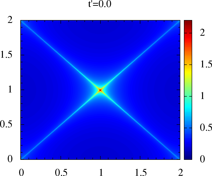
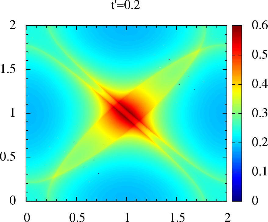
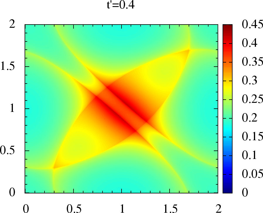
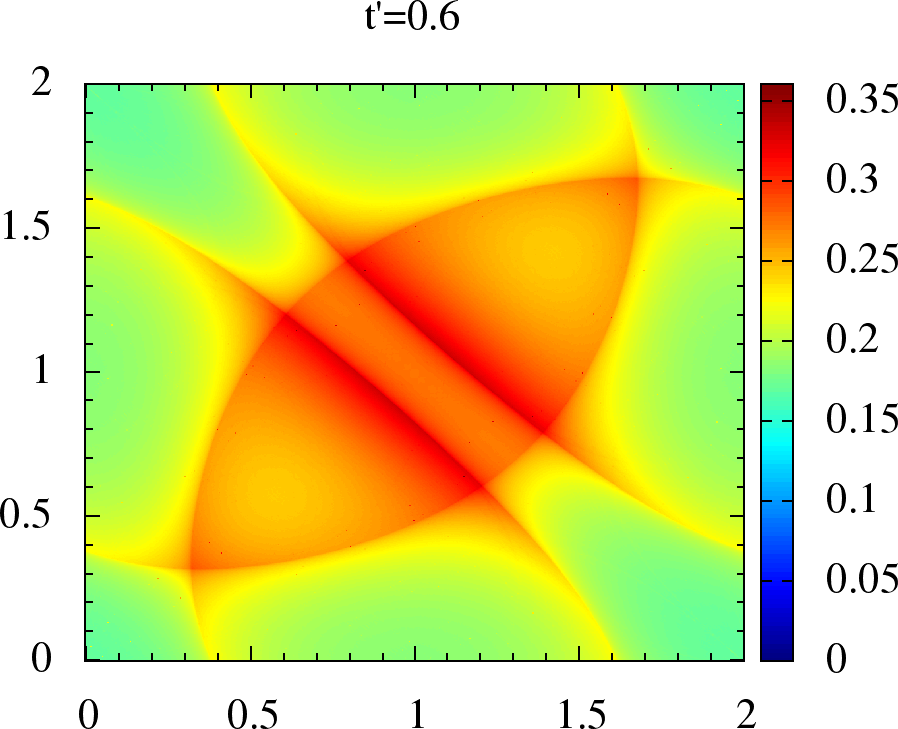
For in the range , the peak in is still at (Figure 2 upper panel) and the system still prefers Neel order but beyond .
For for , however, the maximum shifts significantly away from (Figure 2 lower panel), so, as we will discover, the system may exhibit spiral order.
At strong coupling , the Mott localized phase is described by a Heisenberg model. On the square lattice the resulting order is again at . With growing the progressively more frustrated structure reduces the stability of the Neel state. A spiral state may emerge at large .
At a given , the weak coupling and strong coupling wavevectors are in general not the same.
 |  |  |  |
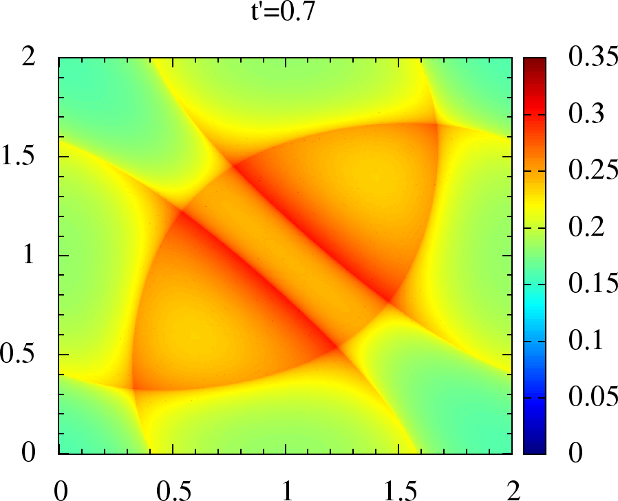 | 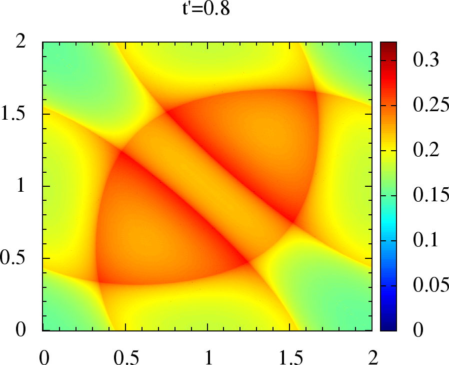 | 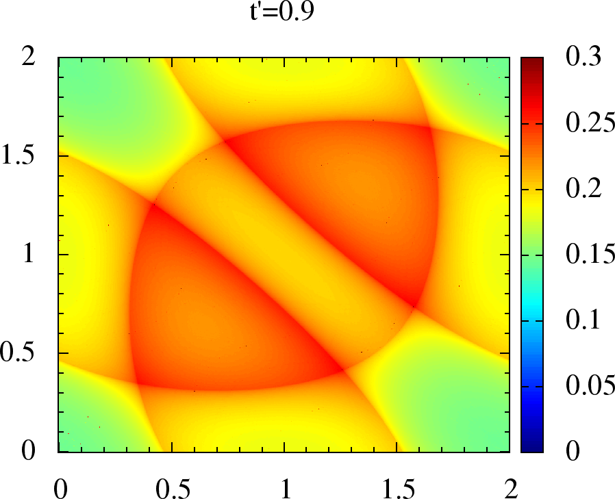 | 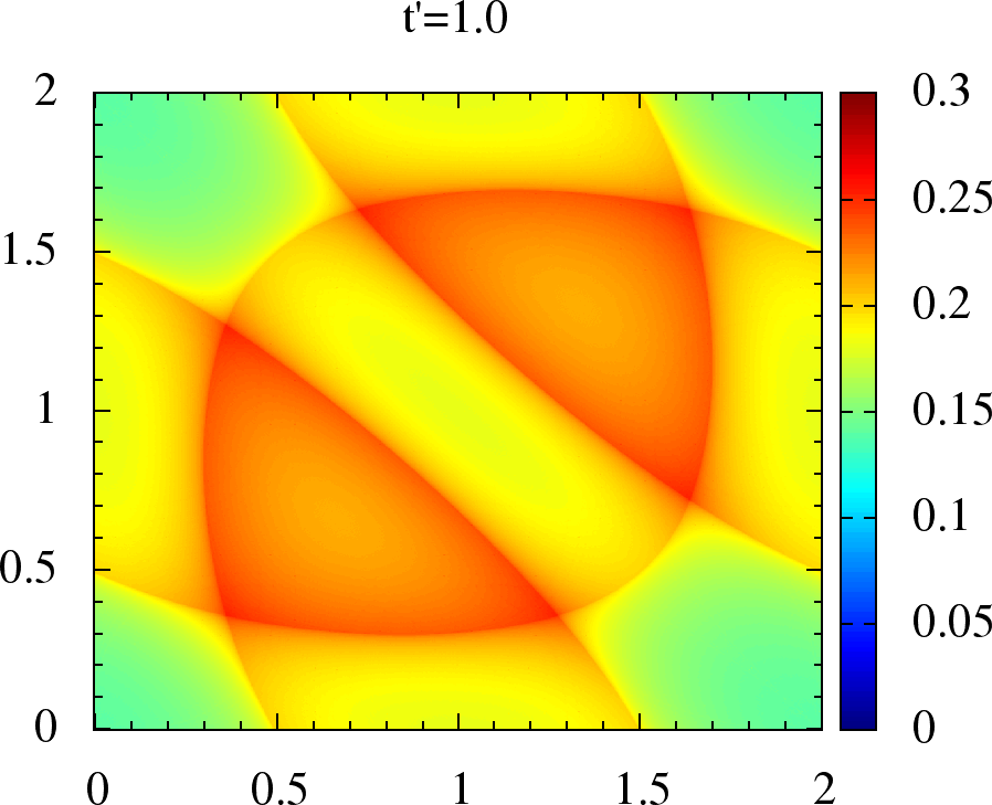 |
Figure 2:Non-interacting magnetic susceptibility for anisotropic triangular lattice. We have , on the and axes, in units of for each plot. The upper panel is for where the maxima lies on, or around , while in lower panel for the maxima has shifted to incommensurate .
So, in contrast to the bipartite case, the dominant magnetic wave vector evolves from to as changes at finite . When is typically incommensurate, as we will see later, it generates smaller gap compared to Neel order (for moments of the same size). This leads to the possibility of a magnetic metal at intermediate coupling.
In a two dimensional system thermal fluctuations prevent long range order at finite temperature, and quantum fluctuations could suppress order even at . Nevertheless an approximate solution of the magnetic problem, retaining classical thermal fluctuations can lead to valuable insight. In the present chapter we provide a comprehensive study of the Hubbard model in the anisotropic triangular lattice in the full range of [0-1] over a wide range of .
We use a real space new approach to the Mott transition, using auxiliary fields, that emphasizes the role of spatial correlations near the metal-insulator transition (MIT). Our principal results, based on a combination of Monte Carlo (MC) on large lattices and variational minimization, are the following.
We establish a ground state magnetic phase diagram in the plane, and explore the finite temperature Mott transition by calculating transport and spectral functions at four representative cross sections of .
The phase diagram is established for selected choice of . For , relevant for the -BEDT compounds, our results bear a strong resemblance to properties measured in these organics.
At intermediate temperature, in the magnetically disordered regime, we obtain a strongly non Drude optical response in the metal, and predict a pseudogap (PG) phase over a wide interaction and temperature window.
The electronic spectral function is anisotropic on the Fermi surface, with both the damping rate and PG formation showing a clear angular dependence arising from coupling to incommensurate magnetic fluctuations.
We start with the Hubbard model defined on the anisotropic triangular lattice, defined as in Figure 1 and use the square lattice geometry with anisotropic hopping for nearest neighbours and for the next nearest neighbours. As discussed in section The Hubbard model, we used Hubbard Stratonovich transformation to decouple the interaction term, and after a sets of approximation, we have the following effective Hamiltonian equivalent to equation (9) for the given hoppings:
We will set as the reference energy scale. corresponds to the square lattice, and to the isotropic triangular lattice. The first two terms are just the tight binding parts for the anisotropic triangular lattice. Third term has constant shift of on-site energy. The last two terms are of crucial importance, in which the first term couples the electrons to the classical fields with coupling , and splits the on-site energy for two spins state by . The magnitude of the field is controlled by the last term. controls the electron density, which we maintain at half-filling, . is the Hubbard repulsion.
2Ground state phase diagram
| (a) | (b) |
|---|---|
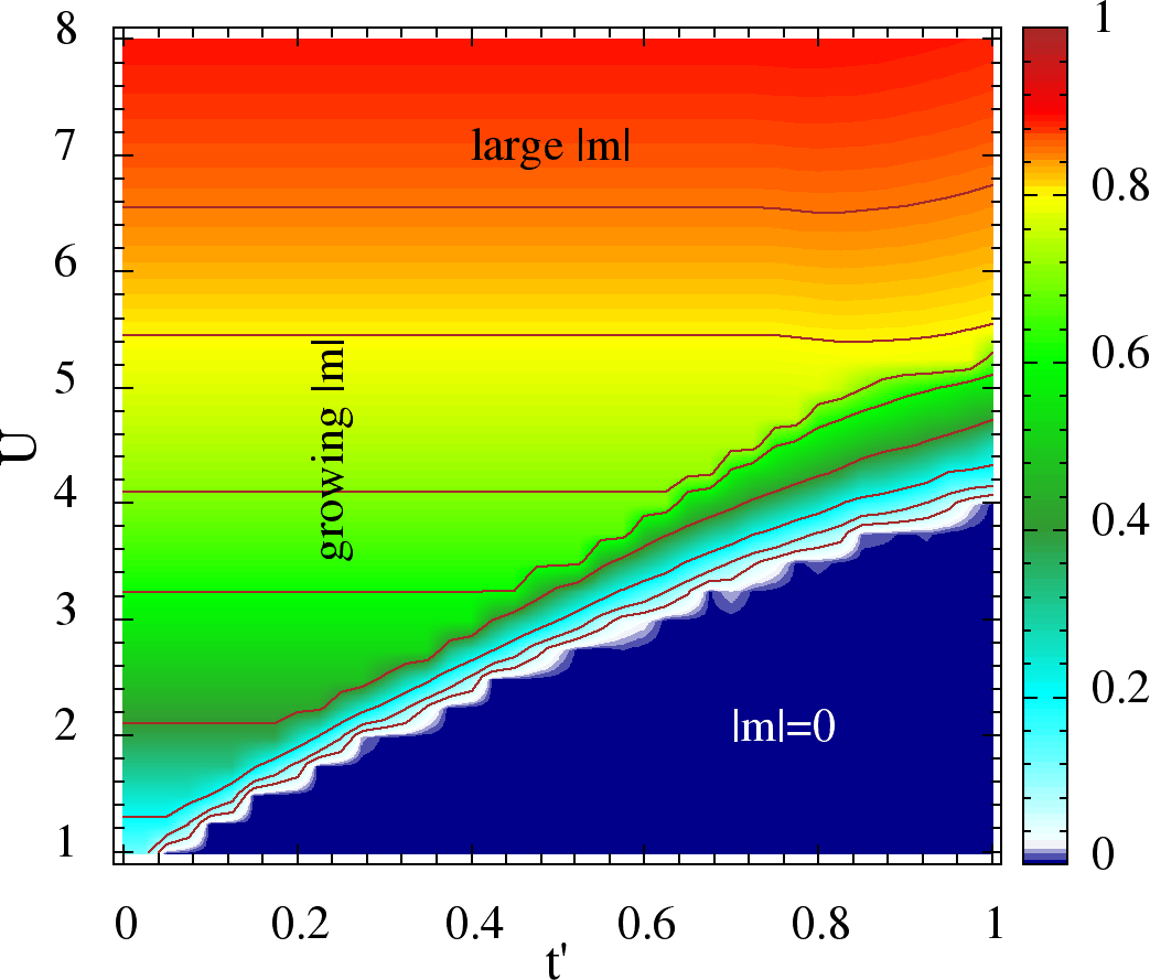 |
Figure 3:Left/Top: The ground state phase diagram. The blue region denotes the Neel state characterized by . The thin red strip along denotes the three sub-lattice 1200 spiral for which . The pink region represents incommensurate spirals at generic . A reduced scale of shown as green arrows is drawn as illustration in the spiral region. The black line is the metal insulator boundary based on gap in the state, so that region below it is gapless/metallic. The lower white portion gives the non-magnetic solution. Right/Bottom: The color plot of the optimal in the plane. The contours are visual guide to constant .
First, let study the ground state (T=0) behaviour of the system for generic value of , and . As mentioned in the section Variational minimization at , in order to get the ground state, one has to minimize the total energy at half filling with respect to the fields. In a brute force minimization, for site lattice, this would result in minimizing a function of variable, which is an N-P hard problem, not to mention that calculation of the energy would involve numerical diagonalization for each field. However, If we look for periodic solutions, the number of parameter to minimize with, becomes small and independent of system size . Motivated by the simplicity to solve and generality, we chose the variational set described by which describes a periodic field configuration, in which the magnitude of the field at each lattice site is , and its angular direction have periodicity of the period vector . Once we restrict to this set, the total energy becomes the function of the magnitude and the period , i.e., . Besides its calculation is fairly easy and we discussed it in section Variational minimization at . For a given , one gets the optimal after minimizing the total energy, which characterizes the electronic nature of the state.
| (a) | (b) | (c) |
|---|---|---|
Figure 4:The magnetic instability wavevector inferred in the weak coupling limit (panel (a)), the corresponding (panel (b)), and the Heisenberg limit wavevector (panel (c)). These results set the rough `analytic’ limits of the theory. A full optimisation based on the MC is needed at intermediate coupling. should fall to zero as , accessing that requires calculation on much bigger lattices.
2.1Magnetic phases
In Figure 3 (top/left) we have shown the ground state phase diagram, which summarizes the magnetic nature of the states in the plane. The primary phases are collinear Neel order (G-type), incommensurate spiral (SP) and three sub-lattice 1200 (at ), which have non zero and solutions. At lower and larger one gets solutions giving uncorrelated metallic (non-magnetic) state. The line stays at Neel order (G-type) for all values upto , which continuously shrinks from the low side following the MIT line, and eventually is destabilized against spirals at . Beyond , we have spiral whose period gradually shifts from to , which is the ground state for large limit for triangular lattice . In fact, at large it shifts along straight line connecting and . The right panel of the figure we have shown the optimal in the plane. At lower , the stays constant in the Neel region, and starts decreasing once in the spiral region, and eventually vanishes. Thus in general, spiral phases have lower as compared to Neel phase at given moderate .
A quick understanding can be obtained by examining the weak coupling and strong coupling limits. Within the RPA scheme the peak in decides the instability, as we have discussed before. Panel (a) in Figure 4 shows this wavevector . Notice that it stays close to for and then shifts quickly. The corresponding is shown in panel (b). These decide the weak instability and magnetic phase. For , deep in the Mott phase the system is a Heisenberg model, and the wavevector for that, labelled is shown in panel (c). Remember that .
The band susceptibility was calculated on sizes upto , but capturing the divergence of as requires much bigger lattices.
2.2Density of states
Figure 5:Density of states of the electron system at , using the variationally minimised background (which is roughly consistent with MC results).
Recalling the tight binding dispersion , and the dispersion, we had for generic spiral state for given and ,
one can easily see that, for (the Neel phase) when . Thus eigenvalues get divided into two sets with , so that the gap at half filling has a lower bound of (which is also the gap). Thus the Neel phase always has a gap for any nonzero value of .
Given the optimised values of and at a given and the density of states can be readily generated. We show such results in Fig.\ref{dos-T0} for four values of , and in all four cases. It shows an insulating (gapped) state at all when , and the presence of a metal - with crossover to an insulating state at the larger cases.
While the specific bandstructure here arises from the presence of long range order in the background, the survival of the large insulator at finite is not related to order at all. The finite temperature discussion will highlight this.
A word about the gap. The expression (min - max) whenever greater than zero, gives the gap at half filling, but is difficult to calculate analytically for general value of and . We have hence numerically calculated the gap for the ground state, which is shown in Figure 6. This suggests that spiral, which have lower values compared to Neel phase, tend to have smaller gap, as a result the metal insulator boundary (shown as black line in the phase diagram in Figure 3) which is the locus of zero gap, has a positive slope with . Thus increasing reduces the insulating character, and if is moderate, carries the system across the insulator to metal transition.
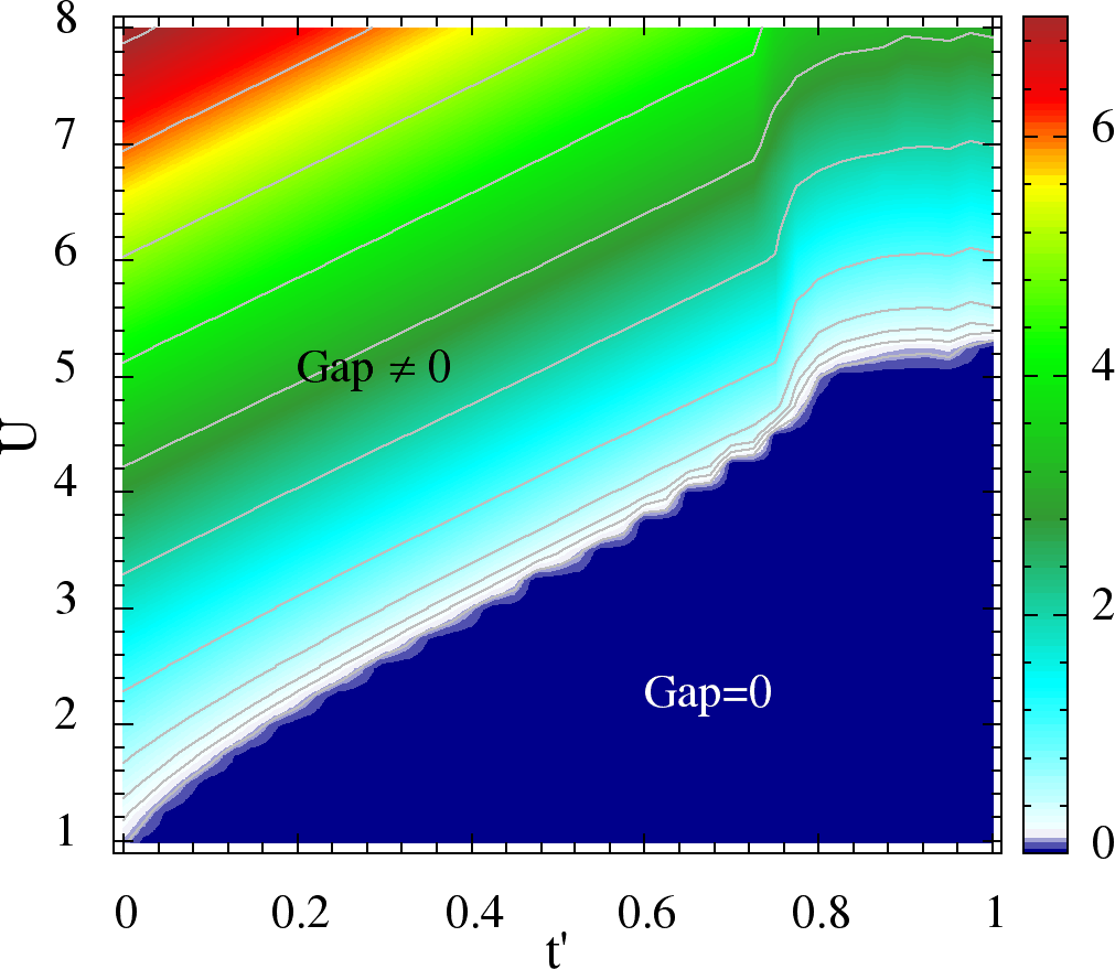
Figure 6:The colour plot of the gap estimated in ground state.
This summarizes the discussion of the ground state. As mentioned in the section Static approximation in the Hubbard model, the effective model we used, reduces to unrestricted Hartree-Fock at , but with no assumption about the translational symmetry. It supports only static moment phases, usually either long range ordered, or non-magnetic (). However, when we raise the temperature from , the exact inclusion of the thermal fluctuations generated via the classical fields, quickly improves the accuracy of the method with increasing temperature. In the next section we discuss the effect of the thermal fluctuations at finite temperature, on the and their impact on electronic properties.
3Finite temperature properties
We accessed the finite temperature physics of the effective model using the real space Monte Carlo sampling discussed in section Real space Monte Carlo, on lattice. The system was annealed from high enough temperature , to in discretized intervals. At each temperature, large number of samples of were generated from the equilibrium distribution.
These were used to analyze the spatial correlation and the ordering tendency of the fields. The electronic properties like density of states, optical conductivity, DC resistivity, spectral function etc., were calculated by taking the thermal average over each of these individual configurations. The system was studied for different degree of hopping anisotropy in the entire range of [0-1], and based the results of magnetic correlations, electronic properties and transport, we mapped out phase diagram.
3.1Phase diagrams
Below, we first summarize our results using phase diagram. Then, we discuss in detail the spatial correlations of the fields in section Section 3.2. Then in the following sections we show how these correlations affect the electronic properties, specifically electronic density of states (section Section 3.4), transport (section Section 3.3), the spectral function and its anisotropy (Section 3.5).
Figure 7:Finite temperature phase diagram, for four values of . (a)~, (b)~, (c)~, (d)~. The phases are paramagnetic metal (PM), paramagnetic insulator (PI), antiferromagnetic metal (AFM) and antiferromagnetic insulator (AFI). In (a), and (b) the AFM and AFI phases are simple Neel ordered, while in (c) and (d) these are non-collinear phases. PG indicates the pseudogap phase. T indicates the temperature at which magnetic correlation length becomes larger than lattice size. The MIT line defines the crossover from metallic to insulating character, based on transport.
In Figure 7, we have shown the interaction()-temperature() phase diagram, drawn at four representative values of . The low temperature result is equivalent to UHF, and leads to a transition from an uncorrelated paramagnetic metal (PM) to an antiferromagnetic metal (AFM) at some , followed by antiferromagnetic insulator (AFI) at some (except when ). For (Figure 7a) and (Figure 7b), the AFI and AFM (for ) is simple Neel ordered, while for (Figure 7c) and (Figure 7d), its non-collinear phase with , and respectively. At , the AFI survives down to , with decreasing moment, and there is , and no AFM phase. The magnitude is small in the AFM phase, and grows as increases in the insulating (Mott) phase. The window of AFM slowly grows upon increasing as seen in the ground state variational phase diagram. However, the existence of the AFM, and the nature of order in the intermediate Mott phase, could be affected by the neglected quantum fluctuations of the .
Finite temperature brings into play the low energy fluctuations of the . The effective model has the symmetry of the parent Hubbard model so it cannot sustain true long range order at finite . However, our annealing results suggest that magnetic correlations grow rapidly below a temperature , and weak inter-planar coupling would stabilize in plane order below (we have checked this explicitly). This scale increases from zero at , reaches a peak at some , and falls beyond as the virtual kinetic energy gain reduces with increasing . The systematically increases with increasing , while the maximum at systematically goes down.
We classify the finite phases as metal or insulator based on the , the temperature derivative of the resistivity. The dotted line indicating the MIT corresponds to the locus . In addition to the magnetic and transport classification we also show a window around the MIT line where the electronic density of states (DOS) has a pseudogap. To the right of this region the DOS has a ‘hard gap’ while to the left it is featureless.
For , the MIT line has a positive slope, which increases with temperature, and at very high temperature, the line becomes nearly vertical. However, for finite it becomes vertical at some moderately hight temperature , after which the slope turns negative, showing re-entrant insulator-metal-insulator behavior with increasing near . We discuss the details of the re-entrance later.
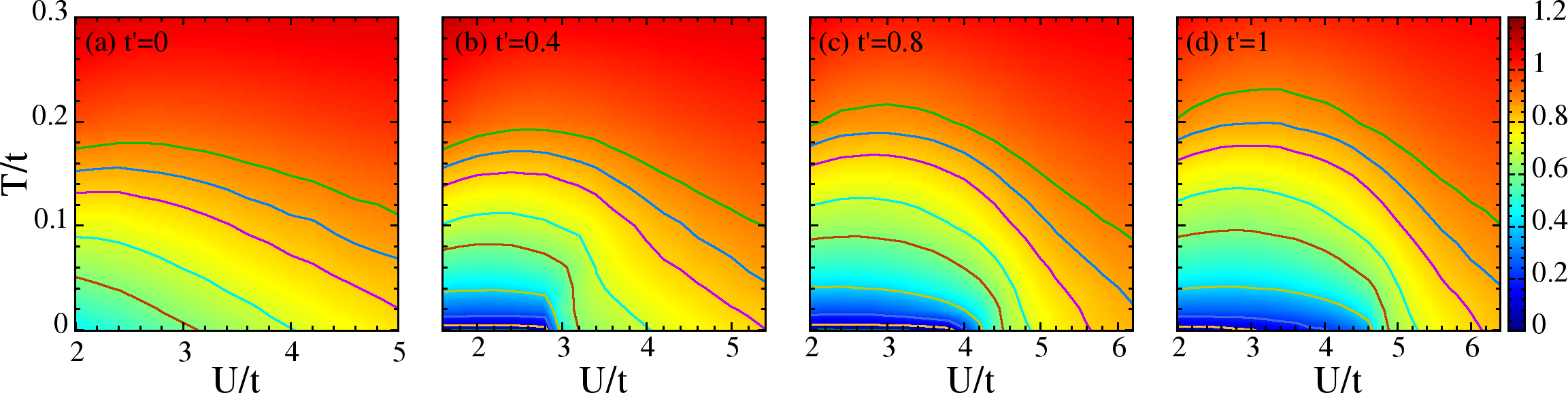
Figure 8:The dependence of for various temperatures, four representative values of . (a) , (b) , (c) and (d) .
3.2Auxiliary field correlations
We saw in the section \ref{sec:gs2d}, that the ground state is either magnetic, with non-zero fixed and corresponding , or non-magnetic with . At finite temperature, the thermal excitations would generate fluctuations in the configurations. This happens by allowing (a) differing magnitudes of the fields at different sites and (b) randomized angles of the . These fluctuations, generate a variety of interesting states, as we saw in the last section. We will now try to see some trends in the nature of these fluctuations, in the plane. As we will see in the subsequent sections, each have a different impact on electronic properties. Thus broadly we have two kind of fluctuations in the :
3.2.1Magnitude distribution
When the ground state had non-zero , and periodic angular variation given by , the excitations would generate states with non-uniform , which will be distributed in some form around the average . At very low temperature, will be very close to the ground state optimal value , and systematically will {\it increase} with temperature. The ground state that had , would now generate non-zero distribution with increasing with temperature. In the Figure 8 we have shown the dependence of at different temperatures for the four representative values of anisotropy . There is systematic increase in with temperature at all and , however the rate of change of is larger in metallic or low . At very high temperature , the becomes nearly independent of .
Figure 9:The magnitude distribution at two values of plotted for values of typical of weak and strong coupling and three temperatures each.
The distribution of these , denoted by (or in short referred to as ) is defined as following
where denotes the Dirac delta function, and denotes the thermal average over equilibrium configurations. Lets see this first for the simplest case of square lattice . In Figure 9 we have shown (a) the temperature dependence of the at a fixed , and (b) the dependence at a fixed temperature. At T=0, will be a delta function peaked at the optimal . It progressively broadens around the mean, , which itself increases with T. The dependence in panel (b) shows that magnitude fluctuations are larger in lower , while larger , or more insulating systems have smaller magnitude fluctuations. This indicates that the angular fluctuation are more crucial in insulating systems. Although we have discussed it in the context of square lattice, these features of magnitude fluctuations are valid for all .
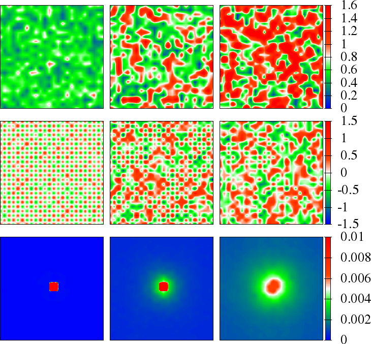
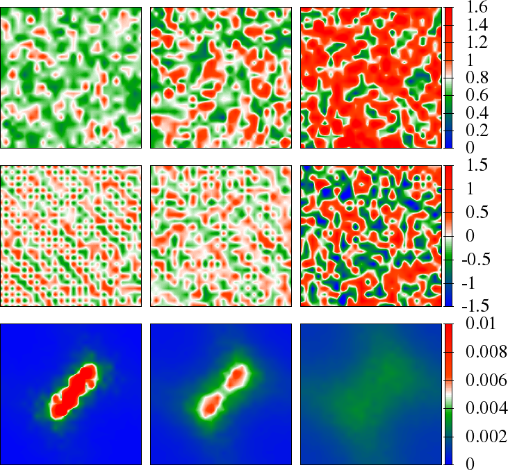
Figure 10:Snapshots of the auxiliary field magnitude, nearest neighbour angular correlation , and the structure factor . The top/left panel is for and (the square lattice with Neel order) and the bottom/right set is for and (anisotropic triangular lattice with spiral order). Top row in each set is , next row is NN , where is a fixed reference site, third row is . Temperatures (from left to right) are .
3.2.2Angular correlations
We calculate the following thermally averaged structure factor to proble angular correlation:
In a state of with completely random angles, the structure factor for all . However, as angles start to get correlated, some of the increase at the cost of other, and the maximum value (at some s) of starts to increase. Upon lowering the temperature, when the system goes under the magnetic transition, the rapid growth of structure factor at some is observed, whose onset temperature defines magnetic transition temperature.
In Figure 10, we have shown the temperature dependence of the structure factor aided with some snapshots of the fields. At very low , the magnitudes almost uniform, their directions alternate in all directions as in Neel state, and the structure factor is sharply peaked at . Progressively, upon increasing T, is fluctuate, angular correlation weakens and the peak value of structure factor reduces, spilling its weight to neighbouring values. The right panel shows similar data on the anisotropic case at where the reference state is now a spiral.
Next, in Figure 11 we have shown the evolution of the snapshots at a fixed temperature for different at . As the interaction strength increases, one observes the increase in the typical values of and decrease in its fluctuations. Simultaneously, the angular correlations become stronger with , evolving from a short range correlation at to progressively better antiferromagnetic states at higher interaction strength ().
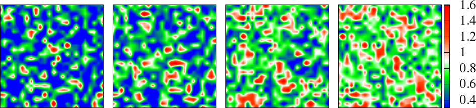
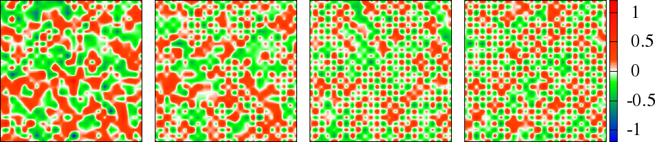
Figure 11:Snapshots of fields showing dependence of magnitude fluctuations and the angular correlation at , , plotted on lattice. Top row: Site dependent magnitude . Bottom row: , where is field at some reference point. The electrons see these as typical configurations, as the system evolves from correlated metal with small to antiferromagnetic insulator with large .
To summarize, based on the results on the known square lattice, we know that, the fluctuations of the field increase with increasing temperature. The magnitude fluctuations are stronger at lower , showing broader compared to large . The angular correlations are stronger in large systems.
The nature of angular correlation becomes more complex, once we go to larger where the ground state has order at incommensurate . In Figure 12 we show the evolution of the structure factor at two temperatures, one at high temperature, and the other close to . First of all, the peaks are not at , but at incommensurate , which the same , at which the ground state orders.
Besides, the spread is is larger compared to what we saw in square lattice at the same temperature. This means stronger angular fluctuations, and lower .
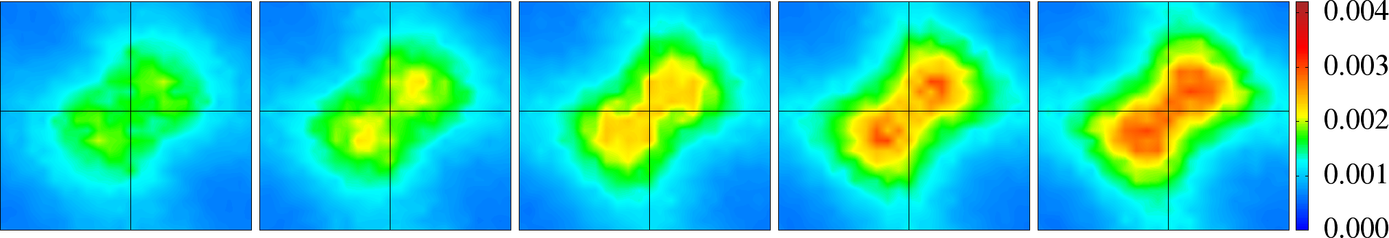
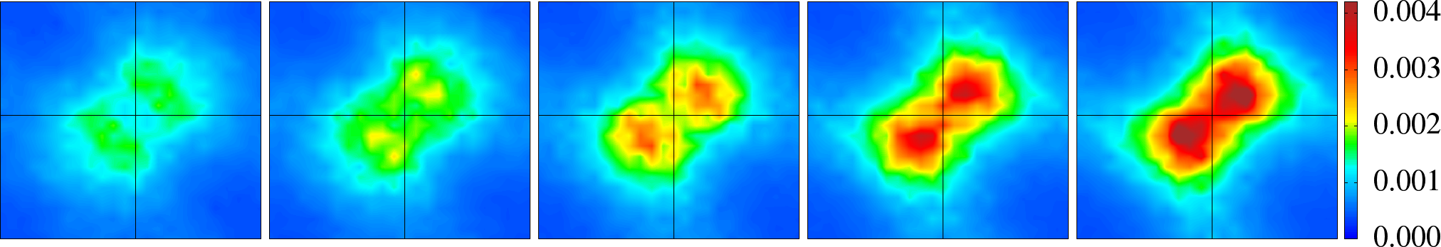
Figure 12:The structure factor for plotted for increasing (left to right), at two temperatures (top row) and (bottom row).
3.3Transport and optical response
For the optical conductivity , and the resistivity , we used the Kubo formula for optical conductivity. In Figure 13 we show the resistivity computed from the Monte Carlo for varying . Our resistivity is in units of , being the lattice spacing.
Figure 13:Temperature dependence of the resistivity for different in the neighbourhood of the MIT, plotted for the same four cross sections of as chosen in Figure 7 (a) , (b) , (c) and (d) . The values, shown here are chosen around the MIT, displayed in the legend. %The normalization scale is .
In a full treatment of the Hubbard model, retaining the quantum fluctuations of , one would expect in the metallic side. This is what DMFT produces, consistent with the experiments. Our resistivity also vanishes as , modulo effects of finite annealing, but is described more by . This is an artifact of the classical approximation (). However, as increases the classical thermal fluctuations should provide an adequate description of the transport.
Figure 14:Temperature evolution of the optical conductivity . The left and right boxes are for , and respectively. The chosen cross sections of are (a) , (b) , (c) and (d) . In each figure, three temperatures are plotted.
In Figure 14, we have shown the temperature evolution of the optical conductivity , for for four values of , and two values of , (left frame) and (right frame). In a Drude metal, the optical conductivity would have maximum at , and quickly loose weight to higher frequency, while in a Mott insulator the optical conductivity would have a gap at low frequency, after which it would pickup weight which would have maxima near . Its easy to see the following trends from the :
In both frames, (a) and (b) i.e., are insulating with no weight at low frequency, and the maxima is peaked around . At low temperature, the gap is larger along the peak value. With increasing the temperature, progressively, the gap is decreased by the transfer of spectral weight at low frequencies, eventually having small Drude weight at high temperature. One can guess that this would correspond to a density of state with weak gap, or strong pseudogap with very low weight near the Fermi level, and the gap in the density of states would diminish, progressively with increasing temperature.
In the left frame (c) and (d), i.e., are metals having large weight at . The peak in is close to in (c) while its exactly at in (d). With increasing temperature, the Drude weight and the peak value decreases, and the peak locations moves to higher . The response at higher temperature, thus becomes non-Drude metal. This would correspond to `weakly correlated metal’ whose density of state, has large weight at Fermi level, which depletes progressively towards higher energies, forming pseudogap.
In the right frame, (c) and (d) i.e., both have vanishing Drude weight, and most of the spectral weight surrounds The low frequency weight slowly increases with higher temperature, and the high weight, center around disperses. This one would expect very close to MIT, on the insulating side where the gap is vanishingly small. The density of state in such case would have very strong dip at Fermi level, with small weight at low energy.
Figure 15:Optical conductivity at (a) , (b) for varying across , for . At these temperatures the is non Drude even in the ‘weakly correlated’ case . The finite frequency peak evolves into the Hubbard transition at large .
In Figure 15, we show the optical conductivity at and as the interaction is varied across the Mott crossover, for . Our first observation is the distinctly non Drude nature of in the metal, , with . The low frequency hump in the bad metal evolves into the inter-band Hubbard peak in the Mott phase. The change in the lineshape with increasing is more prominent in the metal, with the peak location moving outward, and is more modest deep in the insulator.
In the next section, we discuss the trends in the density of states (DOS) of the systems, as function of temperature and the interaction strength, and would explicitly show the trends we have guessed.
3.4Density of states and pseudogap
In Figure 16, we have shown the temperature evolution of the density of state , for the same set of parameters as in the Figure 14. Its easy to see from the low temperature DOS, that (i) in both frames, (a) and (b) i.e., are insulating in the ground state, showing hard gap. (ii) in the left frame (c) and (d), i.e., are good metals, with large DOS at Fermi level. (iii) in the right frame, (c) and (d) i.e., both have strong dip in the DOS at the Fermi level. Evolution to higher temperature, increases the low frequency weight at Fermi level of an insulator, which results in narrowing the gap, and eventually a strong dip pseudogap phase. On the contrary, heating the uncorrelated metal (left frame (c) (d)), depletes the weight at Fermi level, thereby inducing a soft dip pseudogap, which becomes stronger at higher temperature.
Figure 16:Temperature evolution of the DOS . The left and right boxes are for , and respectively. The chosen cross sections of are (a) , (b) , (c) and (d) . In each figure, three temperatures are plotted.
At some fixed temperature, when we increase the interaction , then at some , the magnetic fluctuations become strong enough to induce the pseudogap in the DOS, which deepens progressively with , and at some , would become hard gapped. The local of these and defines the region containing the pseudogap, shown earlier in the finite phase diagrams (Figure 7). The Figure 17 explicitly shows the crossover from the metal to the insulator involving a wide window of pseudogap, where the pseudogap window widens with increasing temperature. Here we have taken , and chosen the range across the MIT. One can see, that at (Figure 17(a)) that has a small dip at Fermi level (close to ), and is on the verge of hard gap. At higher temperature (Figure 17(b)), the dip in the has increased, while has slowly gained some spectral weight.
In general, in the region between the line and the MIT line, the dip feature deepens with with , and we have , while in the region between MIT and we have weak . The PG arises from the coupling of electrons to the fluctuating . A large at all sites would open a Mott gap, independent of any order among the moments. Weaker , thermally generated in the metal near and with only short range correlations, manages to deplete low frequency weight without opening a gap. Since the typical size increases with in the metal, we see the dip deepening at .
In Figure 18, we show the map of DOS at the Fermi level over the entire plane, at temperatures , showing the evolution from the hight DOS in the metal to the vanishing DOS in the Mott phase through low finite DOS in the PG phase.
Figure 17:Density of states at for varying across . The dip in the DOS deepens with increasing for . For larger the system slowly gains spectral weight with increasing .
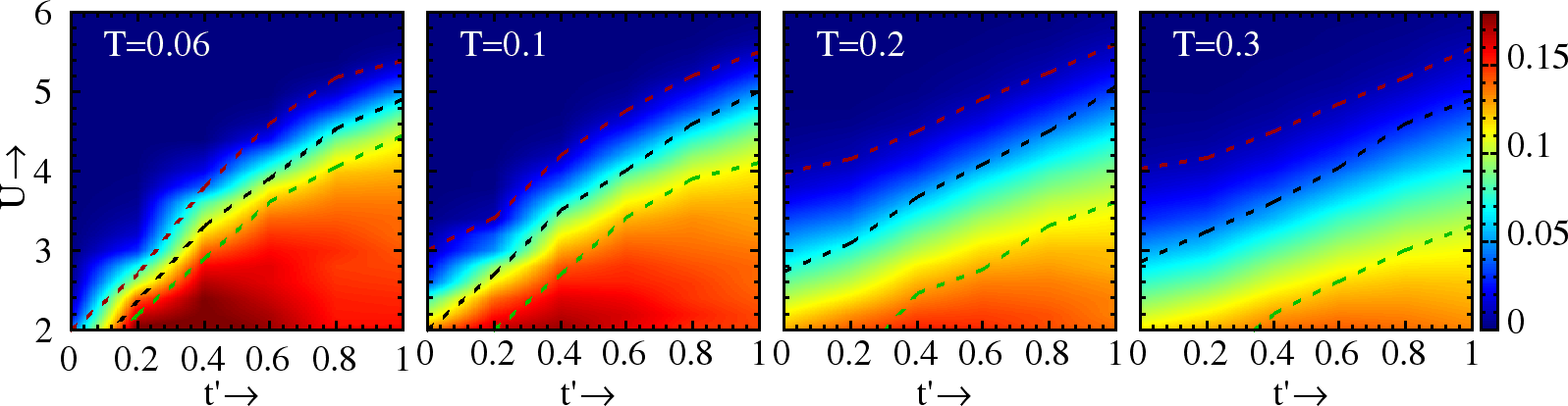
Figure 18:Map of the , the DOS at Fermi level, in the plane at four temperatures . The black dotted line denotes the MIT crossover. The region between red and green dotted line represents the pseudogap region.
3.5Angle resolved spectral functions
While the size of the determine the overall depletion of DOS near and the opening of the Mott gap, the angular correlations dictate the momentum dependence of the spin averaged electronic spectral function
Within a ‘local self energy’ picture, as in DMFT, should have no dependence on the Fermi surface (FS). In that case we should have a independent suppression of with increasing . However, inclusion of spatial fluctuations would be able to access the dependence of the spectral function.
Below we first show the evolution of the , across the Mott transition, in connection with the angular correlations through the structure factor . We discuss two limiting cases (a) the square lattice in Figure 19, where the angular fluctuations are strong near , and (b) in Figure 20, where they are at incommensurate~(0.85,0.85). In both figures data is shown, and are chosen near the metal insulator crossover.
![t'=0 case. Top: Momentum dependence of the low frequency spectral weight in the electronic spectral function A({\bf k},\omega) at T/t=0.1. k_x,k_y range from [-\pi,\pi] in the panels. Note the systematically larger weight near {\bf k} = [\pi/2,\pi/2] and symmetry related points and smaller weight in the segments near [\pi,0] and [0,\pi] and symmetry related points. U/t=2.0,~2.2,~2.4,~2.6,~2.8, left to right. Bottom: S({\bf q}) for the {\bf m}_i fields for the same set of U/t. The q_x,q_y range from [0,2\pi]. Note the very weak structure at U/t=2.0 and the much larger and much sharper peak at U/t=2.8.](/thesis/build/ak_T0p1_tp0p0-7177dbd9e690f69c721cbf68a9ad0f96.png)
![t'=0 case. Top: Momentum dependence of the low frequency spectral weight in the electronic spectral function A({\bf k},\omega) at T/t=0.1. k_x,k_y range from [-\pi,\pi] in the panels. Note the systematically larger weight near {\bf k} = [\pi/2,\pi/2] and symmetry related points and smaller weight in the segments near [\pi,0] and [0,\pi] and symmetry related points. U/t=2.0,~2.2,~2.4,~2.6,~2.8, left to right. Bottom: S({\bf q}) for the {\bf m}_i fields for the same set of U/t. The q_x,q_y range from [0,2\pi]. Note the very weak structure at U/t=2.0 and the much larger and much sharper peak at U/t=2.8.](/thesis/build/sq_T0p1_tp0p0-b84c063f251ac521789da129093bb6c5.png)
Figure 19: case. Top: Momentum dependence of the low frequency spectral weight in the electronic spectral function at . range from [-] in the panels. Note the systematically larger weight near and symmetry related points and smaller weight in the segments near and and symmetry related points. , left to right. Bottom: for the fields for the same set of . The range from . Note the very weak structure at and the much larger and much sharper peak at .
![Top: Momentum dependence of the low frequency spectral weight in the electronic spectral function A({\bf k}, \omega) at T/t=0.1. k_x,k_y range from [-\pi,\pi] in the panels. Note the systematically larger weight near {\bf k} = [\pi/2,\pi/2] and [-\pi/2,-\pi/2] and smaller weight in the segments near [\pi,0] and [0,\pi]. U/t=4.2,~4.4,~4.6,~4.8,~5.0, left to right. Bottom: Magnetic structure factor S({\bf q}) for the auxiliary fields {\bf m}_i for the same set of U/t. The q_x,q_y range from [0,2\pi]. Note the very weak and diffuse structure at U/t=4.2 and the much larger and differentiated structure at U/t=5.0.](/myst_assets_folder./figures/mott_tri/ak_T0p1.png)
![Top: Momentum dependence of the low frequency spectral weight in the electronic spectral function A({\bf k}, \omega) at T/t=0.1. k_x,k_y range from [-\pi,\pi] in the panels. Note the systematically larger weight near {\bf k} = [\pi/2,\pi/2] and [-\pi/2,-\pi/2] and smaller weight in the segments near [\pi,0] and [0,\pi]. U/t=4.2,~4.4,~4.6,~4.8,~5.0, left to right. Bottom: Magnetic structure factor S({\bf q}) for the auxiliary fields {\bf m}_i for the same set of U/t. The q_x,q_y range from [0,2\pi]. Note the very weak and diffuse structure at U/t=4.2 and the much larger and differentiated structure at U/t=5.0.](/thesis/build/sq_T0p1-b01f767a7eb32d375018c748d10545b6.png)
Figure 20:Top: Momentum dependence of the low frequency spectral weight in the electronic spectral function at . range from [-] in the panels. Note the systematically larger weight near and and smaller weight in the segments near and . , left to right. Bottom: Magnetic structure factor for the auxiliary fields for the same set of . The range from . Note the very weak and diffuse structure at and the much larger and differentiated structure at .
In both figures, the top row shows maps of for , as increasing transforms the bad metal to a Mott insulator. The first panel at for (a) and for (b) shows weak anisotropy on the nominal Fermi surface. The Fermi is square for , while elliptical in shape for with minor axis along direction. At the next panel, the weak anisotropy is much amplified and the weight in the direction is distinctly larger.
Figure 21::height: 9.2cm :width: 13.0cm
Angle resolved spectral functions and highlighting the behaviour at the ‘hot’ and ‘cold’ spot on the Fermi surface.
The next three panels basically show insulating states but without a hard Mott gap. Overall, the ‘hot spot’ where destruction of the Fermi surface seems to start is at , for the case, while the same for is near It ends near the ‘cold spot’, where the Fermi surface is strongest. The cold spot is near , for , and around for . With increasing the PG feature would form at the hot spot while the cold spot would still have a quasi-particle peak.
The second row in Figure 19, Figure 20 shows the structure factor of the fields at for the same as in the upper row. For the system is some what below , as a result magnetic correlation is large, hence the structure factor is quite sharp, around , even though the order hasn’t fully developed. For , however, there is no magnetic order as the system is quite above its . Still, we can see the growth of correlations centered around as increases. The dominant electron scattering would be from to , and the impact would be greatest in regions of the Fermi surface in the proximity of minima in . The location of the hot spots on the Fermi surface, and the momentum connecting them, indeed correspond to this scenario.
Figure 22:Angle resolved spectral functions and and as is increased across the Mott transition.
Figure 21 shows the full spectral function at the two points on the Fermi surface where the spectral weight is either maximum (labelled ) or minimum (labelled ). The results are shown for but are generic as far as crossover from a correlated metal to a Mott insulator are concerned. Notice the suppression of a broad ‘quasiparticle’ feature, visible at low , as the interaction strength is increased, and the emergence of a pseudogap. The occurence of the pseudogap itself requires a magnetically disordered state, and could have been captured by a tool like DMFT. The anisotropy on the Fermi surface, however, arises from the momentum dependence of the self energy and requires a method that retains spatial correlations.
Figure 22 shows the spectral function for a complete momentum sweep across the Brillouin zone, as the system is taken across the finite temperature Mott crossover. In the left panel a quasiparticle peak is visible at all while in the middle panel there is a pseudogap in the spectral functions (a clear two peak structure) as crosses the Fermi level. This gets more prominent in the right panel.
3.6Reentrant metal-insulator transition
In this section, we focus on an unusual reentrant feature in the phase diagram. We focus on and will comment on other parameter values at the end. Our main results on this issue are the following:
We observe that on the anisotropic triangular lattice there is indeed a window of interaction strength , beyond the zero temperature metal-insulator transition at ,where the resistivity shows an insulator-metal-insulator (I-M-I) crossover with increasing temperature.
The density of states (DOS) at the Fermi level also has non monotonic behaviour with temperature, and the two crossover scales and in the resistivity can be correlated with the behaviour of the DOS.
We relate the re-entrance to two competing effects in the underlying model and observe that re-entrance is absent on the square lattice, and is only weakly visible in the fully isotropic triangular lattice.
For the primary features are: (i) the transition from a paramagnetic metal (PM) to an antiferromagnetic metal (AFM) ground state at and then a transition to an antiferromagnetic insulator (AFI) at , (ii) an increase in the magnetic correlation scale, from to and then a gradual decrease, and (iii) a wide pseudogap window around the finite temperature MIT line. Since we are interested in the metal-insulator transition and its salient features, we will identify with and focus on a narrow window around it.
Figure 23:Temperature dependence of resistivity, for interaction in a narrow window around . The values of are displayed besides the curves.
Figure 23 show the resistivity in the narrow window of near the transition. We use this as our primary indicator of metallic or insulating behaviour. When we call the system metallic, when we call it insulating. Beyond the metal-insulator transition at the DOS in the ground state shows a finite gap. The resistivity shows the following features:
For the resistivity increases monotonically with increasing .
For the resistivity first decreases with increasing upto the insulator-metal crossover temperature, , increases from till the metal-insulator crossover , and then decreases slowly.
For the resistivity decreases monotonically with temperature. The two scales and are shown further on in the phase diagram.
Figure 24:Temperature dependence of the DOS at three typical interaction strengths. Top: monotonic suppression of the low energy DOS with increasing temperature in the metal at . Middle: non monotonic behaviour of the low energy DOS with at , in the insulator-metal-insulator crossover window. Bottom: monotonic increase in the low energy DOS with increasing `deep’ in the insulator at .
Figure 24 shows the temperature dependence of the low energy DOS at three representative interaction strengths.
The top panel shows the behaviour at where the ground state is metallic. In this case the DOS at the lowest temperature, is featureless, but increasing temperature leads to the appearance of a progressively sharper dip near . This is a regime of pseudogap formation due to strong magnetic fluctuations in metal, but remains positive at all . The DOS at the Fermi level falls almost to of its value on raising the temperature to .
The middle panel shows the DOS at where the ground state is insulating and the resistivity shows a thermally driven I-M-I crossover. At the lowest temperature that we show, , there is a dip in the low energy density of states (up from a weak Mott gap at ). The low frequency DOS gains weight till , not surprising in a weak insulator, beyond which there is sustained decrease of low energy weight.
The bottom panel shows the behaviour deeper in the insulating regime . Here the resistivity decreases monotonically with (the highest in Figure 23 is but the similar behaviour holds at larger as well). The system starts with a hard gap at which fills up slowly with increasing . Even at the highest temperature the DOS is less than 10% of the non-interacting value.
Figure 25(a) shows the DOS at the Fermi level for varying interaction strength and temperature. The two metallic cases, and 4.2 show monotonic decrease of with . The insulating cases have at . They gain weight with increasing , have a peak at some temperature and then decrease as in the metallic cases. For much beyond the re-entrance window, would rise (exponentially) slowly and monotonically with . We have not shown that regime here.
Figure 25:(a) Temperature dependence of the density of states at the Fermi level, , for varying . (b) : the average of the density of states over the low frequency window around . Since the DOS has a sharp frequency dependence in the re-entrance window we think the low frequency average, rather than just , provides a better correspondence with transport.
The principal lesson from Figure 24 and Figure 25 is the non monotonic temperature dependence of the low energy density of states, in a manner that complements the resistivity behaviour. Figure 25(b) shows , the density of states averaged over temperature dependent low frequency, defined by
Since the DOS has a sharp feature near , we feel this frequency averaged quantity, rather than itself, may have a better correspondence with the conductivity. In fact, while falls sharply with even at , flattens out, with a hint of increase at high at large .
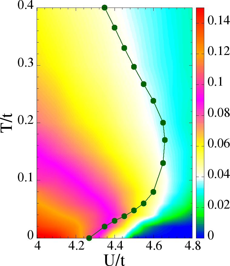
Figure 26:Top/Left: Phase diagram emphasizing the re-entrant feature near . The MIT line, , is the locus . In the lower part, it indicates thermally driven IM crossover, which matches the T (blue squares) reasonably (see text). Its upper part, indicates a MI crossover. Bottom/Right: a colour plot of , with the line superposed. There is reasonable match between the shapes of constant contour and that of .
Figure 26 shows the metal-insulator phase diagram and the associated thermal crossover scales. The ground state is an antiferromagnetic (spiral) metal for , and an antiferromagnetic insulator for . The magnetic ‘transition temperature’ increases with in the interval shown, and falls again for . The MIT line has re-entrant character, we label the lower part, with , as and the upper part, with , as . One can see the from Figure 26 (left) that curve matches reasonably with , while from Figure 26 (right) we see that more or less follows constant low frequency DOS contour.
![Top/Left: P(m) distribution at U=4.2 (metal), 4.5 (re-entrance window) and 5.4 (insulator) and T=0,0.06,0.1,0.2 . Bottom/Right: The structure factor S({\bf q}) arising from the spatial correlation of the {\bf m}_i at same U values and T=0.1,0.2 . The q_x,q_y axes in the color plots are in range [0,2\pi], so the center is (\pi,\pi).](/thesis/build/sq-reent-7925977458cc50cea55d05a7662c13e5.png)
Figure 27:Top/Left: distribution at =4.2 (metal), 4.5 (re-entrance window) and 5.4 (insulator) and T=0,0.06,0.1,0.2 . Bottom/Right: The structure factor arising from the spatial correlation of the at same values and T=0.1,0.2 . The axes in the color plots are in range [0,2], so the center is (,).
In Figure 27, we have shown the distribution of the magnitude of fields (left) and the structure factor (right) at few temperatures and three representative values 4.2 (in the metal), 4.5 (in the re-entrant region) and 5.4 (in the insulator). The distribution shows the growth of the mean value with at low , and as we go to higher T, the distribution becomes more and more broader, and eventually all start looking the same at very high temperature. The plot demonstrates how angular correlations grow stronger with increasing , and weaker with increasing temperature. At low T, shows peak around =(0.85,0.85) and its conjugate , which corresponds to a non-collinear `spiral’ AF state. The closer the peak is to (,) (G-type phase), the stronger is the AF nature of the phase, and the sharper the peak, the stronger is the AF correlation.
In what follows we first try to create an understanding of the re-entrant feature in terms of the behaviour of the microscopic variables . We will then compare our results to CDMFT, and finally with the experimental situation.
The transport behaviour in Figure 23 is obviously correlated with the behaviour of the density of states seen in Figure 24 and Figure 25. The phase diagram and the associated contour plot for in Figure 26 makes this correspondence more explicit. This allows us to shift focus to the behaviour of the low energy DOS, and analyze it in terms of the mean, variance, and angular correlation of the .
We would like to address three questions: (i) why is there a maximum in , how does it correlate with ? (ii) what determines the dependence and the downward trend in beyond ?, and (iii) why is there another M-I crossover at higher temperature?
It can be shown (at least numerically) that
When the is sharply peaked, increasing AF correlations tends to increase the gap in the DOS.
For given AF configuration, the gap increases with increasing
For a given strength of AF correlation, broadening of tends to vanish the gap.
Its the competition between these mechanisms, which leads to the re-entrant behaviour, as we argue below.
Since the moments are AF ordered at low , this leads to a growing spectral gap and a stronger insulating state with increasing . With increasing the broaden and the mean value also increase. If the AF pattern had remained rigid with increasing this would have strengthened the insulating state. However, the magnitude fluctuation and the angular randomness lead to a broadening of the spectrum, weakening of the gap, and growth in .
Beyond the angular disorder almost saturates and the slow growth of with , leads to a loss of low energy spectral weight in both in the metallic and insulating samples. The peak in therefore arises from a competition of growing (tending to suppress ) and growing randomness (that enhances ).
4Comparison with experiments
We saw in the previous sections, that triangular structure leads to frustrating magnetic interaction in the insulating phase. However, even if long range order is lost, short range spin correlations still have dramatical affect on the electronic properties near the MIT. The organic salts we mentioned in the section Section 5.2, provide a concrete test bed for this effect (Kanoda & Kato (2011), Powell & McKenzie (2011)). The (BEDT-TTF)Cu[N(CN)]-X salts are quasi two dimensional (2D) materials where the BEDT-TTF dimers define a triangular lattice with anisotropic hopping (Kandpal & others (2009)). The large lattice spacing, , leads to a low bandwidth, resulting in large . For the XClBr family the frustration is moderate and a magnetically ordered state with K for is obtained(Lefebvre & others (2000), Kagawa et al. (2004)). The low temperature state is an AFI for and metallic for (with a superconducting (SC) instability at K). The PM state is very incoherent above K: the resistivity \cite{org-res} is large, mcm, the optical response has non Drude character (Merino & others (2008), Dumm & others (2009)), and NMR (Powell et al. (2009), Kawamoto et al. (1995)) suggests the presence of a pseudogap (PG). The detailed spectral features of this unusual state are not known.
In this section we attempt to connect the results of the triangular lattice Mott physics with available experiments on the ClBr family. We first, choose the electronic hopping parameters suggested, by ab initio calculations, and earliar theoretical attempts. We choose primary hopping meV (Kandpal & others (2009)), and . This would convert temperature expressed in units of to that in Kelvin.
4.1Parameter estimation
If we pretend, that applying ‘pressure’ or, in the present context, increasing the Br doping , only reduces , not , then we have as function of . For simplicity we will now denote as . The only one unknown now is the dependence of the interaction on . In the ClBr family it is observed that the transport gap can be fitted to Kelvin(Yasin & others (2011)), and for -Cl, upon pressure, it can be fitted to (Limelette & others (2003)). We match this to the dependence of our calculated gap, , and infer , where our calculated gap matches with the experiment. The MIT occurs at and for us at . We used a quadratic polynomial fit for , and found that reproduces the transport gap(Yasin & others (2011)) estimated from the resistivity experiments. A similar fit is constructed for the hydrostatic pressure. The comparison is shown in Figure 28. The range in resistivity in Figure 13(c) corresponds roughly to . Since meV, is approximately 300K.
Figure 28::width: 6.0cm :height: 5.0cm
Comparison of the experimental and fitted Mott gap.
4.2Optical conductivity
The conductivity of the two dimensional system is first calculated as follows (ref. Allen (2006)), using the Kubo formula:
Where, the current operator is
The d.c. conductivity is the limit of the result above. =, the scale for two dimensional conductivity, has the dimension of conductance. is the Fermi function, and and are respectively the single particle eigenvalues and eigenstates of in a given background {}.
Figure 29:Comparison of the experimental and theoretical optical conductivity near the Mott transition. The experimental data at is extracted from Fig.3 of Dumm et al Dumm & others (2009).
The experimental results are quoted as resistivity of a three dimensional material. If we assume that the planes are electronically decoupled then the three dimensional resistivity can be estimated from the resistance of a cube of size . If the 2D resistivity is , the resistance of a sheet is just itself. A stacking of such sheets, with spacing in the third direction, implies that the resistance of the system would be . By definition this also equals . Equating the two, . Recalling that the normalizing scale for the resistivity was . Using , we have cm for the organics.
The absolute magnitude of our metallic resistivity at is about mcm, while the experimental value is mcm(Yasin & others (2011)). The difference could arise from electron-phonon scattering which is absent in our model. Limelette et al Limelette & others (2003) presented a DMFT based resistivity result that compares favourably with experiments, but, apparently, involves an arbitrary scale factor.
We showed the dependence of the optical conductivity in Figure 15, at . For a rough comparison to organics, 80K, cm, and cm.
Figure 30:Comparison of the estimated and experimental .
In the organics the experimenters have carefully isolated the Mott-Hubbard features in the spectrum by removing phononic and intra-dimer effects (Dumm & others (2009)). Since we have already fixed our we have no further fitting parameter for . The measured spectrum at and K has a peak around cm. Using and we get , which translates to cm. The magnitude of our at is cm, since cm. This is remarkably close to the measured value, cm (Ref. Dumm & others (2009) Fig.3). In Figure 29, we have shown the temperature evolution of the optical conductivity near the Mott transition. In the ClBr the transition occurs around , while for us, it occurs around , or .
While the characteristic scales in match well with experiments, the experimental spectrum has weaker dependence on temperature and composition . This could arise from the subtraction process and the presence of other interactions in the real material. Our result differs from DMFT (Merino & others (2008)), and agrees with the experiments, in that we do not have any feature at . We have verified the f-sum rule numerically.
4.3Transition temperature
Finite temperature brings into play the low energy fluctuations of the . The effective model has the symmetry of the parent Hubbard model so it cannot sustain true long range order at finite . However, our annealing results suggest that magnetic correlations grow rapidly below a temperature , and weak inter-planar coupling would stabilize in plane order below . This scale increases from zero at , reaches a peak at , and falls beyond as the virtual kinetic energy gain reduces with increasing (Figure 7(c)).
Since at , from our results this would indicate that , at , i.e, K, not too far from the NMR inferred K. In Figure 30 we show a comparison of the experimental and the .
4.4Reentrant M-I transition
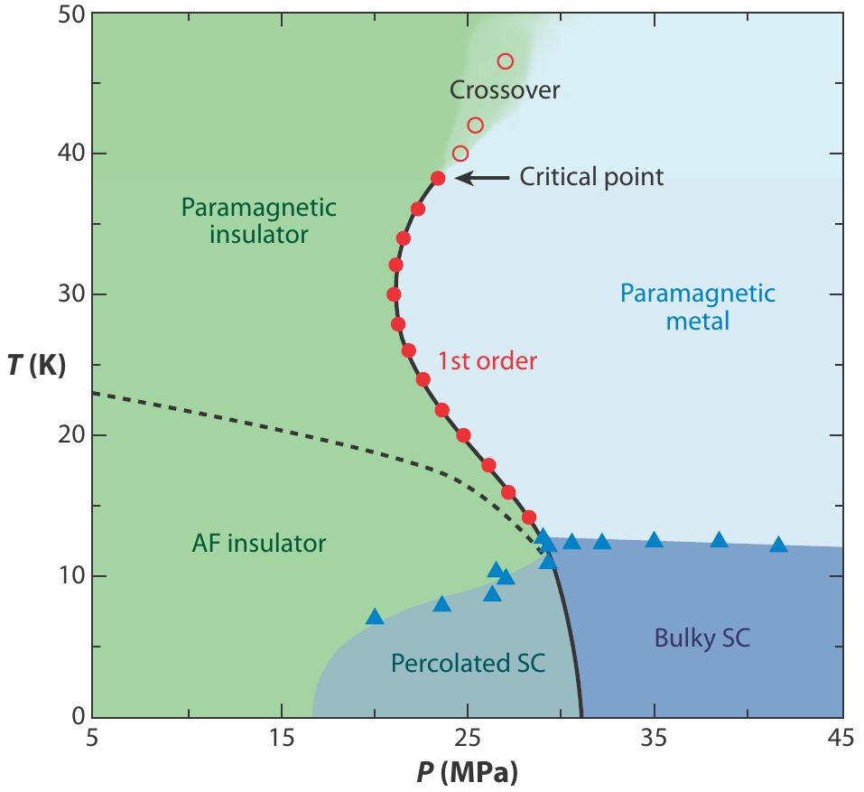
Figure 31:Comparison of the phase diagram with experiment.
In the organics of the (BEDT-TTF)Cu[N(CN)]-X family in particular one observes an insulator-metal transition (IMT) in the ground state of the XClBr family at , and also a pressure driven IMT when X=Cl(Kanoda & Kato (2011), Powell & McKenzie (2011)). While the increase in bandwidth, and so a decrease in the effective interaction, with increasing the ‘pressure’ is not unexpected, finite temperature brings to life an unusual re-entrance(Limelette & others (2003), Yasin & others (2011)). Over a narrow pressure window (10Mpa), the insulating ground state ‘metallises’ with increasing temperature and then crosses over again to insulating behaviour at a higher temperature. In Figure 31, we show a comparison of the theory reentrance window with that of Kanoda et al(Kanoda & Kato (2011)). For metals or insulators far from the critical interaction the behaviour is monotonic: metals show an increasing resistivity, while insulators show a decreasing resistivity with increasing temperature.
Cellular dynamical mean field theory (C-DMFT) studies suggest that geometric frustration could be responsible for the re-entrance effect that is observed (Ohashi et al. (2008), Liebsch et al. (2009)). The specific predictions about interaction and temperature window, however, seem to vary widely with choice of the DMFT solver, and most of conclusions are based on the behaviour of the ‘double occupancy’ rather than the measurable transport and spectral features.
Our re-entrant window near , inferred from thermally driven I-M-I crossover, is equivalent to . This is consistent with in the ClBr family (Yasin & others (2011)). The C-DMFT estimates of the re-entrant window varies widely, from (Liebsch et al. (2009)) to~ (Ohashi et al. (2008)).
4.5Density of states
We saw, in Section 3.4 that, the crossover from the bad metal to the insulator involves a wide window with a pseudogap in the electronic DOS, . One may have guessed this from the depleting low frequency weight in , Figure 17 makes this feature explicit. We are not aware of tunneling studies in the organics, but the presence of a pseudogap has been inferred from NMR measurements(Powell et al. (2009)). Our results indicate a wide window, , where there is a distinct pseudogap in the global DOS. This suggests that the entire window in the organics should have a PG. For the dip feature deepens with increasing , we have (compare panels (a) and (b), Figure 17), while for we have a weak . The PG arises from the coupling of electrons to the fluctuating . A large at all sites would open a Mott gap, independent of any order among the moments. Weaker , thermally generated in the metal near and with only short range correlations, manages to deplete low frequency weight without opening a gap. Since the typical size increases with in the metal, we see the dip deepening at .
5Conclusions
We have explored in detail a method which retains the spatial correlations that are crucial near the Mott transition on a frustrated lattice. Using electronic parameters that describe the -BEDT based organics we obtain a magnetic , metal-insulator phase diagram, and optical response that reproduces the key experimental scales. We uncover a wide pseudogap regime near the MIT, and predict distinct signatures of the incommensurate magnetic fluctuations in the angle resolved photoemission spectrum.
While the ‘higher temperature’ results are likely to be a good approximant to the full quantum treatment, future work would involve a check on the stability of the unusual magnetic ground states to quantum fluctuations. The absolute value of is also likely to be renormalised upward somewhat if further quantum effects are incorporated.
- Mott, N. F. (1990). Metal-Insulator Transitions. Taylor.
- Kanoda, K., & Kato, R. (2011). Annu. Rev. Condens. Matter Physics., 2, 167.
- Powell, B. J., & McKenzie, R. H. (2011). Rep. Prog. Phys., 74, 056501.
- Kandpal, H. C., & others. (2009). Phys. Rev. Lett., 103, 067004.
- Lefebvre, S., & others. (2000). Phys. Rev. Lett., 85, 5420.
- Kagawa, F., Itou, T., Miyagawa, K., & Kanoda, K. (2004). Phys. Rev. B., 69, 064511.
- Merino, J., & others. (2008). Phys. Rev. Lett., 100, 086404.
- Dumm, M., & others. (2009). Phys. Rev. B., 79, 195106.
- Powell, B. J., Yusuf, E., & McKenzie, R. H. (2009). Phys. Rev. B., 80, 054505.
- Kawamoto, A., Miyagawa, K., Nakazawa, Y., & Kanoda, K. (1995). Phys. Rev. B., 52, 15522.
- Yasin, S., & others. (2011). Eur. Phys. J. B., 79, 383.
- Limelette, P., & others. (2003). Phys. Rev. Lett., 91, 016401.
- Allen, P. B. (2006). Conceptual Foundation of Materials V.2 (S. G. Louie & M. L. Cohen, Eds.). Elsevier.
- Ohashi, T., Momoi, T., Tsunetsugu, H., & Kawakami, N. (2008). Phys. Rev. Lett., 100, 076402.
- Liebsch, A., Ishida, H., & Merino, J. (2009). Phys. Rev. B., 79, 195108.