Non-Collinear magnetic order in the double perovskite
1Introduction
In this chapter we discuss magnetism in the metallic double perovskites ABBO. These involve a transition metal ion B, with a large magnetic moment, and a non magnetic ion B. While many double perovskites (DP) in this category are ferromagnetic there are hints of antiferromagnetic phases at higher electron doping. These are driven by electron delocalisation, instead of the short range superexchange seen in magnetic insulators.
We will present a comprehensive study of the magnetic ground state and scales of the minimal double perovskite model in three dimensions, using a combination of spin-fermion Monte Carlo and variational calculations. The model is defined on the three dimensional cubic lattice, where B and B sites are in a rock salt pattern (Figure 1). The sublattice of the magnetic B atoms is face centered cubic (FCC) and geometrically disallows a Neel state. As a result, the antiferromagnetic tendency manifests itself as spiral order, or non-coplanar ‘flux’ like phases. We will map out the possible magnetic phases for varying electron density, the level separation between the B and B’ ions, and the crucial B-B (next neighbour) hopping .
Figure 1:Left/Up: The lattice structure of the ordered double perovskite ABBO. Right/Down: The same structure with oxygen removed, shows how B-B sites are arranged in rock-salt ordering. If the bottom corner (blue) atom is B, then its B nearest neighbours (connected by blue lines) are also nearest neighbours of each other. The triangles preclude Neel order.
Previous study of double perovskites in two dimensions (Sanyal & Majumdar (2009)) revealed three collinear phases, namely ferromagnet (FM), a diagonal stripe phase (FM lines coupled antiferromagnetically) and a ‘G type’ phase (up spin surrounded by down and vice versa). In 2D the B sublattice is square and bipartite, so there is no frustration. If we had a 3D simple cubic B lattice the counterparts of the 2D phases would be FM, A type (planar), C type (line like) and G type (Neel). The B ion lattice in 3D is FCC, so, while the FM and planar (A type) phases can exist, the C type phase is modified and the G type phase is disallowed.
Figure 1b indicates why it is impossible to have an ‘up’ () B ion to be surrounded by only ‘down’ () B ions, i.e., the G type arrangement. Two B neighbours of a B ion are also neighbours of each other, frustrating G type order. The suppression of the G type phase, which occupies a wide window in 2D, requires us to move beyond collinear phases in constructing the phase diagram for 3D. We will discuss the variational family in Section Section 1.1.
Using a combination of Monte Carlo and variational minimization, our main results are the following:
We map out the magnetic ground state at large Hund’s coupling for varying electron density and B-B level separation. In addition to FM, and collinear A and C type order, the phase diagram includes large regions of non-collinear ‘flux’ and spiral phases and windows of phase separation.
Modest BB hopping leads to significant shift in the phase boundaries, and “particle-hole asymmetry”.
We provide an estimate of the of these phases from the Monte Carlo where possible, or make a rough estimate based an energy difference calculation.
This chapter is organized as follows. In section Section 1.1 we define the effective single band model for the metallic double perovskites and describe the methods we use. Section Section 2 discusses our results on the particle-hole symmetric model, and section Section 3 describes the effect of a introducing electron hopping between the non-magnetic sites. Section Section 4 discusses some issues of modeling the real double perovskites. We summarize and conclude the chapter in section Paragraph.
1.1Effective single band model
The alternating arrangement of B and B ions in the ordered cubic double perovskites is shown in Figure 1. We use the following one band model on that structure:
The correspond to the B ions and the to the B. and are ‘on-site’ energy on the B and B sites respectively, e.g., the level energy of Fe and Mo in SFMO. is the chemical potential and is the total electron number operator. is the hopping amplitude between nearest neighbour B and B ions. We augment this model later to study first neighbour BB hopping as well (). arises from the Hund’s coupling on the shell. The Hund’s coupling itself keeps the 5 core electrons polarised into a state, and the exclusion principle forces the conduction electron spin to be antiparallel to this core spin. We will use , and absorb the magnitude of in . are the Pauli matrices.
The model has parameters , , , and (or ). Since only the level difference matters, we set . We have set , and use so that the conduction electron spin at the B site is slaved to the core spin orientation. The B site levels are shifted to due to the strong on site coupling. To keep the difference between the lower B level and the B level finite we set the parameter , where remains finite even as . We explore the phases as a function of and . We will present results for
() the nearest neighbour hopping model () and
() when a non-zero B-B hopping is introduced.
Figure 2:Level scheme and schematic band structure for the DP model when only B-B hopping is allowed. The arrows denote localized atomic levels. Red and blue denote and spins respectively. The atomic level scheme is shown in (a). where the spin degenerate B levels are at and the spin split B levels are at . We define the effective B level as . When , the levels at and hybridize to create bands, shown for the FM case in (a), and for a collinear AF phase in (b).
A schematic for the on-site levels, and how they hybridize, is shown in Figure 2. The structural unit cell of the system has 2 atoms (one B, one B), which amounts to 4 atomic levels (2 up spin, 2 down spin). The two spin levels at the B site are separated by and overlap with 2 spin degenerate levels of the B site at . We take in the range (0-10). One B band become centered at and second goes to . In this situation the down spin B and two B bands overlap while up spin B band is always empty. The accessible electron density window includes the lowest three bands, so our electron density will be in the range per formula unit.
To get a general feel of the band structure of the particle hole symmetric case, we notice that we have three levels (excluding the highest level at which remains empty and is redundant for our purpose) in atomic limit. These include one spin slaved level at , and the two , , levels which overlap with the levels depending on the spin configurations. This overlap leads to electron delocalisation and band formation.
In the ferromagnetic case, Figure 2(a), only one spin channel (say ) gets to delocalize through sites and forms two bands, separated by a band gap of , while other spin state (say ) is localized at 0.
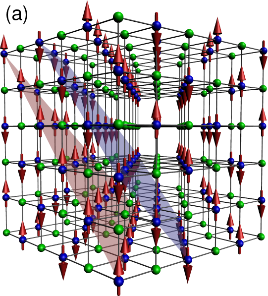
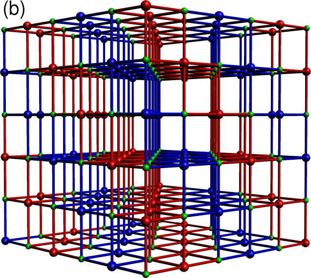
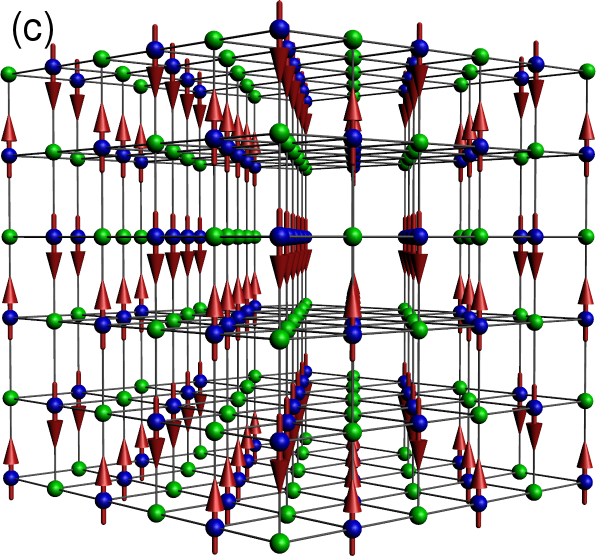
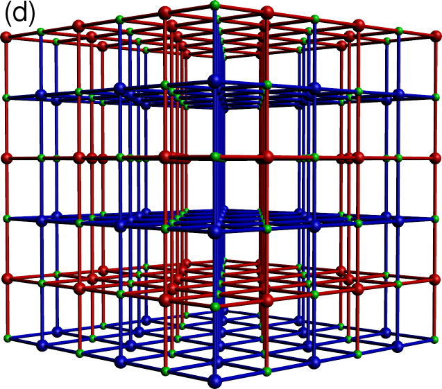
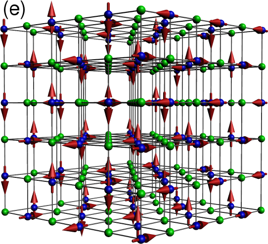
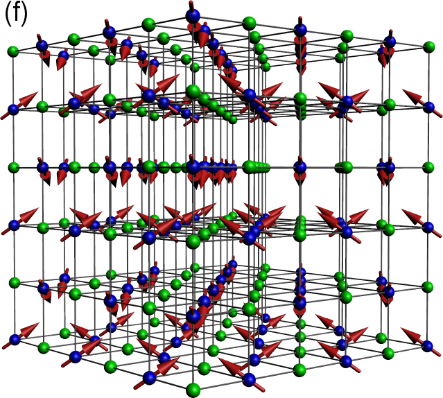
Figure 3:Core spin order, and corresponding electron delocalisation path. (a). ‘A type’ order: the spins are parallel within the 111 planes (shown) and anti-parallel between neighbouring planes. (b) The blue and red bonds show the electron delocalisation pathway for up and down spin electrons in the A type phase. The path is effectively two dimensional. (c) ‘C type’ phase with the spins parallel on alternating 110 planes, and anti-parallel on neighbouring planes. (d) The delocalisation path, consisting of the 110 planes and the horizontal 001 planes. (e) A typical spiral phase and (f) the ‘flux’ phase. Since the spin configurations are non-collinear the electrons delocalize over the whole system.
For collinear AF configurations, the rough band scheme is as shown in Figure 2(b). The conduction path gets divided into two sublattices, such that each spin channel gets to delocalize in one sublattice (in which all the core spins point in same direction, making the sublattice ferromagnetic.) See Figure 3(a)-(b), and Figure 3(c)-(d) for the details of the conduction path. In one such sublattice, only one of the or delocalized, the other remains localized. The roles of and are reversed in going from one sublattice to other, as a result one gets spin-degenerate localized and dispersive bands for AF phases.
1.2Methods of solution
1.2.1Monte Carlo
The model involves spins and fermions, and if the spins are ‘large’, , they can be approximated as classical. This should be reasonable in materials like SFMO where . Even in the classical limit these spins are annealed variables and their ground state or thermal fluctuations have to be accessed via iterative diagonalization of the electronic Hamiltonian. As mentioned in chapter Section 1, we use a cluster based Monte Carlo (MC) method where the cost of a spin update is estimated via a small cluster Hamiltonian instead of diagonalizing the whole system (Kumar & Majumdar (2006)). We typically use a system with the energy cost of a move estimated via a cluster built around the reference site.
We principally track the magnetic structure factor to explore the nature of magnetic order
where denote thermal average. Although the magnetic lattice is FCC, the electrons delocalize on the combined B-B system which is a cubic lattice. Hence we define our wavenumbers with respect to the full B-B lattice. As a result even a simple state like the ferromagnet corresponds to peaks at and and not just . This is because the spin field is also defined on B sites and it has to have zeros value on these sites.
The possibility of complex order in the ground state the Monte Carlo may require large annealing time, and involve noisy data. So, to complement the MC results we have also used a variational scheme discussed below.
1.2.2Variational scheme
We now move to the variational approach. The variational states that we consider here are more complicated than that discussed in the last chapter, and are in number, so we need some caution in implementing the scheme. We compute the energy for periodic configurations where,
with and with if and if . , etc., are unit vectors in the corresponding directions.
The vector field is characterized by the two wavevectors and . For a periodic configuration, these should be and , where ’s and ’s are integers, each of which take values in . There are ordered magnetic configurations possible, within this family, on a simple cubic lattice of linear dimension .
The use of symmetries, e.g., permuting components of , etc., reduces the number of candidates somewhat, but they still scale as . For a general combination of the eigenvalues of H cannot be analytically obtained because of the non trivial mixing of electronic momentum states. We have to resort to a real space diagonalization. The Hamiltonian matrix size is (where ) and the diagonalization cost is . So, an exhaustive comparison of energies based on real space diagonalization costs , possible only for .
We have adopted two strategies:
i. we have pushed this `’ scheme to large sizes via a selection process described below, and
ii. for a few collinear configurations, where Fourier transformation leads to a small matrix, we have compared energies on sizes .
First, scheme (i). For we compare the energies of all possible phases, to locate the optimal pair for each . We then consider a larger system with a set of states in the neighbourhood of . If we consider variation about each component of , {\it etc}, that involves 36 states. The shortcoming of this method is that it explores only a restricted neighbourhood, dictated by the small size result. We have used within this scheme.
Table 1:Candidate phases, the associated , for the spirals, and the peak locations in the structure factor . All the {\bf q} components have the same saturation value, given by , where is the number of non-zero {\bf q} peaks in the S({\bf q}). for FM, A and C, for and SP, for flux and for SP and SP. The factor of comes as we have half the spins at zero value, which halves the normalization.
| Phase | Peak location in |
|---|---|
| FM | (0,0,0),(,,) |
| A-type | (,,),(,,) |
| C-type | (0,0,),(,,0) |
| Flux | , |
| phase | |
| SP: | |
| SP: | |
| SP: | |
The phases that emerge as a result of the above process are (i) FM, (ii) A-type, (iii) C-type, (iv) ‘flux’, and (v) three spirals SP, SP, SP. A-type consists of () FM planes with alternate planes having opposite spin orientation (see Figure 3a). If we convert each of these planes to alternating FM lines, so that the overall spin texture is alternating FM lines in all directions, we get C-type phase (see Figure 3c).
The ‘flux’ phase is different from the spiral families described using period vectors . It is the augmented version of ‘flux’ phase used in cubic lattice double exchange model by Alonso et al (Table-I of ref. Alonso et al. (2001)). It has spin-ice like structure, and is described by
The spiral SP phases are characterized by commensurate values of (See Table 1 for details of periods and the S(q) peaks).
The simplest, SP can be viewed as -angle pitch in the , and directions. The other two spirals SP and SP are respectively C-type and A-type modulations upon SP. Just as flipping alternate planes in a FM leads to the A type phase, flipping the spins in the planes alternatively in SP, leads to SP. Analogously, flipping FM lines in a FM and leads to C-type order - and a similar exercise on SP leads to SP. This modulation is also seen in the peaks of SP and SP. See the Table 1, where all the three spirals have 4 S({\bf q}) peaks common, and SP and SP possess extra S({\bf q}) peaks of the A-type and C-type correlations.
In scheme (ii) we take collinear phases that occur in the phase diagram and compare their energy on very large lattices. This does not require real space diagonalization. The simple periodicity of these phases leads to coupling between only a few states. The resulting small matrix can be diagonalized and the eigenvalues summed numerically. We also included the ‘flux’ phase in this comparison. The details of this calculation, and the the magnetic phase diagram from comparison of FM, A, C and flux phases on large lattice size is discussed in Appendix Section 1.1.
Particle hole symmetry in the model: The electrons move on the cubic lattice divided into two FCC sublattices each of consists of only B or B sites. For each of these sublattice, one can define particle-hole transformation (Fazekas (1999)) as and . This transforms the Hamiltonian as
When , this simplifies to
This symmetry reflects in the phase diagram as the repetition of the phases after half-filling. Introducing the hopping destroys this symmetry, but a reduced symmetry still remains, which relates
This is reflected in the phase diagrams of particle-hole asymmetric case.
2Results: nearest neighbour model
We now discuss the results in the particle-hole symmetric case, i.e, . The situation is discussed in the next section. For each of these cases we first discuss the ground state phase diagram, then the nature of magnetic correlations at finite temperature, and finally the estimate of .
Although the MC approach is ‘unbiased’, the results are are affected by finite size and the use of single spin based update. We use MC results to establish the dominant magnetic correlations in a parameter window and then explore these more carefully using the variational scheme. The MC based estimate is also checked against a rough energy difference calculation that be implemented on the variational ground state.
2.1Monte Carlo
We studied a system using the cluster based update scheme. We used a large but finite to avoid explicitly projecting out any electronic states (undefined (n.d.)), since that complicates the Hamiltonian matrix but allows only a small increase in system size. The magnetic phases were explored for and 10.
Figure 4:Magnetic ground state for varying electron density, , and effective B-B level separation, for the model with only BB, i.e., nearest neighbour, hopping. The labels are: F (ferromagnet), A (planar phase), C (line like), FL (‘flux’) and SP (spiral). This figure does not show the narrow windows of phase separation in the model. The phase diagrams are generated via a combination of Monte Carlo and variational calculations on lattices of size up-to .
In Figure 4, the magnetic ground state is shown, obtained via a combination of Monte Carlo and variational calculations. We see that the phase diagram is symmetric in density. For small , in the range , we have FM, followed by A-type, C-type, and ‘flux’ phase. The order reverses as we go in the other half of the density window. The G-type phase which was largest stable phase in 2D (Fig.2 and Fig.5 in Ref. (Sanyal & Majumdar (2009))) is almost taken over by the ‘flux’ phase. The stability of the ‘flux’ phase decreases with and it does not show up for . The phases that dominate the phase diagram are listed in table Table 1.
Table 2:Peak location in the structure factors for the four A-type phases
| Phase | Plane normal | |
|---|---|---|
| A | ( 1, 1, 1) | (,,)+(,,) |
| A | ( 1,-1, 1) | (,,)+(,,) |
| A | ( 1, 1,-1) | (,,)+(,,) |
| A | (-1, 1, 1) | (,,)+(,,) |
Two complications arise in the Monte Carlo approach in the present model.
i. Additional degeneracy of some AF phases: In addition to the usual spin rotation symmetry, the A-type and C-type phases have four fold degeneracy. The A-type phase for example can arise from planes that are normal to any of the four body diagonals (not just (111)). This leads to growth of domains with different orientation as the system is cooled and multiple peaks in the structure, Table 2.
ii. Geometrical frustration leads to the presence of multiple minima with similar energy and increases the equilibriation time.
| (a) | (b) | (c) |
|---|---|---|
Figure 5:Temperature dependence of structure factor peaks for three typical densities and . (a). The ferromagnetic order at for . (b). The growth of A type correlations (and the noise around the principal peak) at . The ordering wavevector is listed in Table 1. are (c). ‘Flux’ type correlations at . The features are at and around the ordering wavevector in Table 1. Note the scale factors on the axis in (b) and (c).
An illustrative plot of peak features in as function of temperature , is shown in Figure 5 for some typical densities. For FM, S() shows monotonic decrease of T with increasing . For A-type and ‘flux’ phase, the S(q) data shows a number of sub-dominant q peaks whose number keeps increasing as we move to more complicated phases with increasing density. These sub-dominant peaks arise due to a combination of geometrical frustration and our cluster based update.
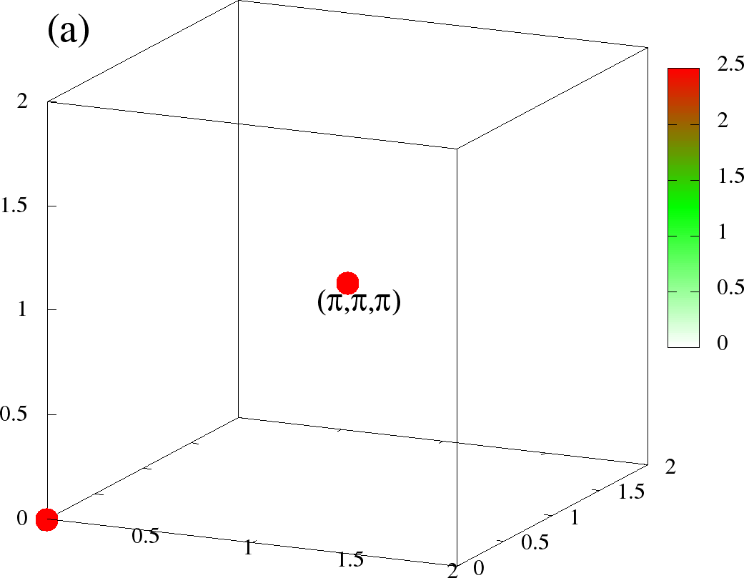
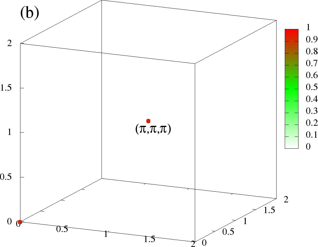
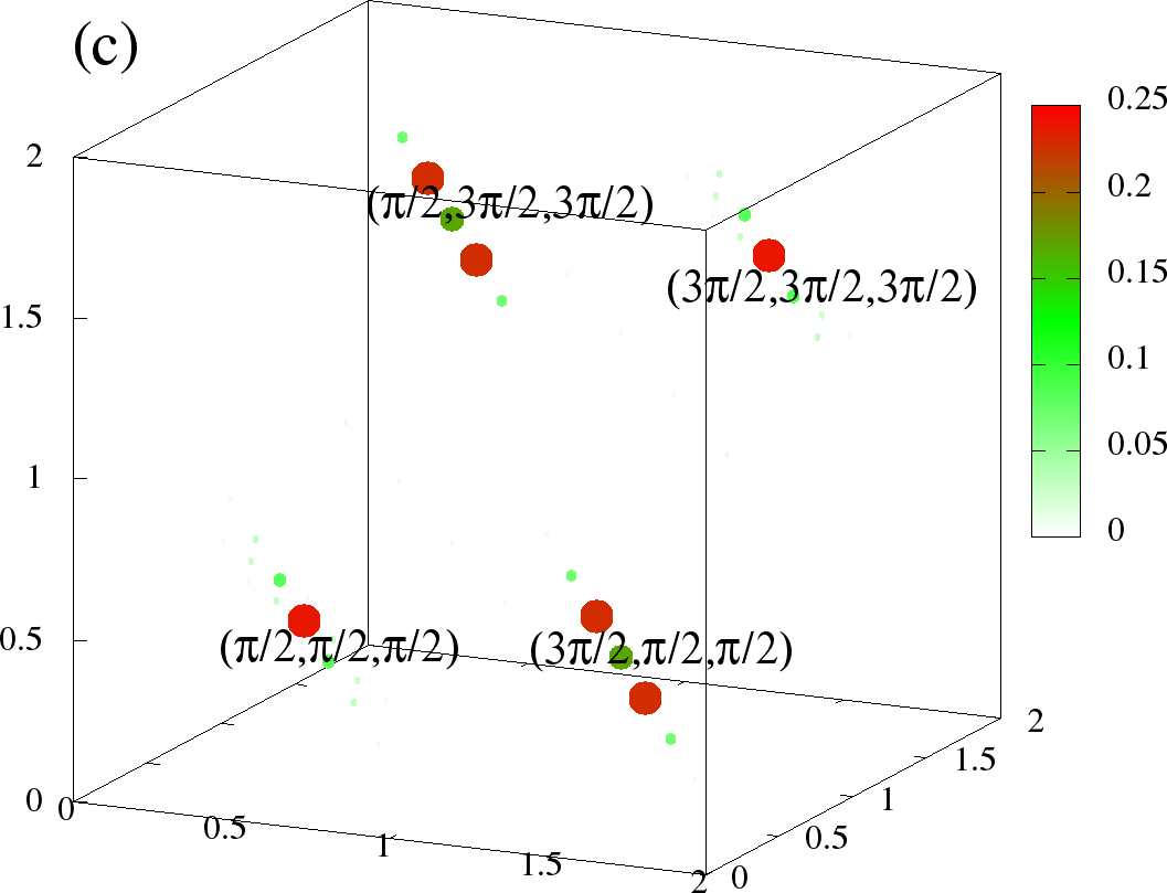
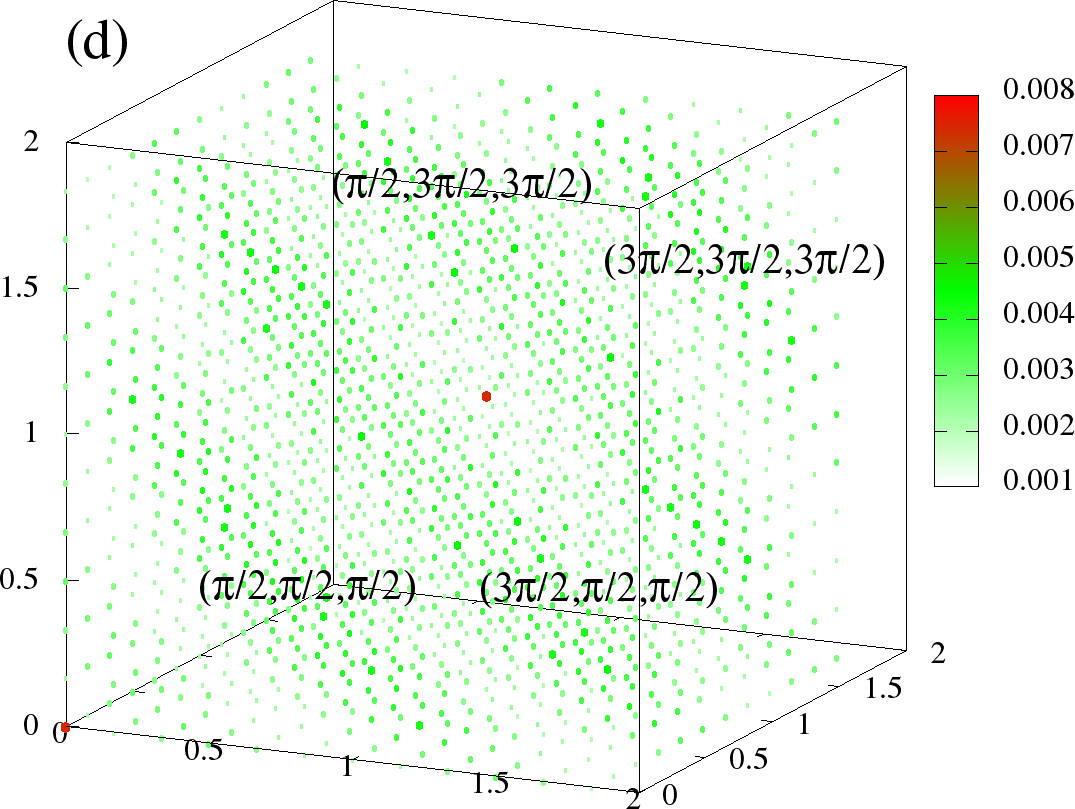
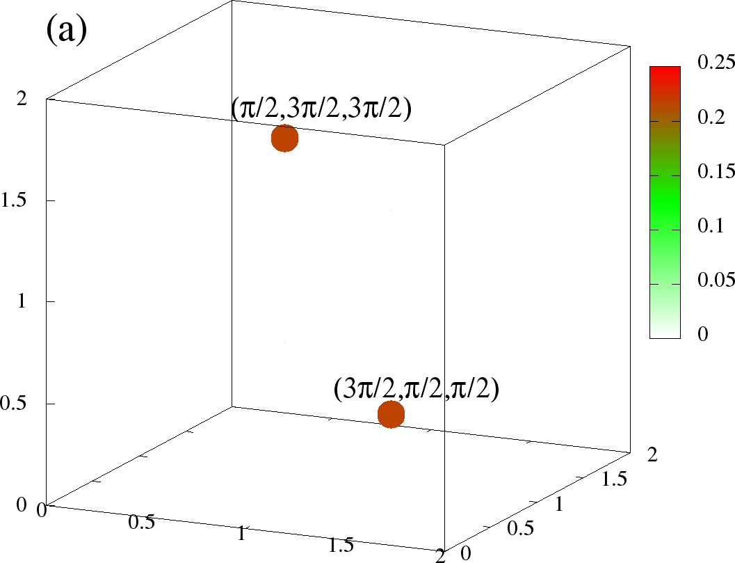
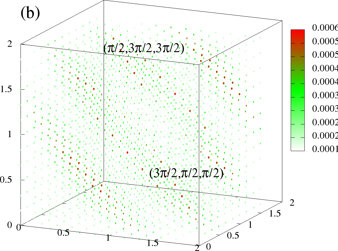
In Figure 6 we show the full structure factor in the the three phases, namely FM, A-type and flux like. The data is visualized in following scheme. At every , a sphere is drawn, whose size, and colour scales with the value of . The colour scheme has white colour for the low values of , so that in the present scheme, only the most prominent are displayed, and the smaller ones are essentially invisible.
| Low T | High T |
|---|---|
 |  |
 |  |
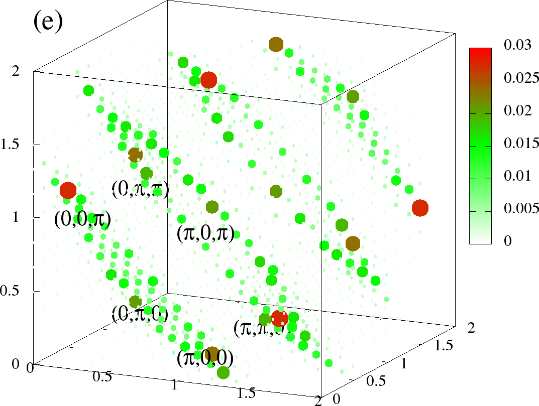 | 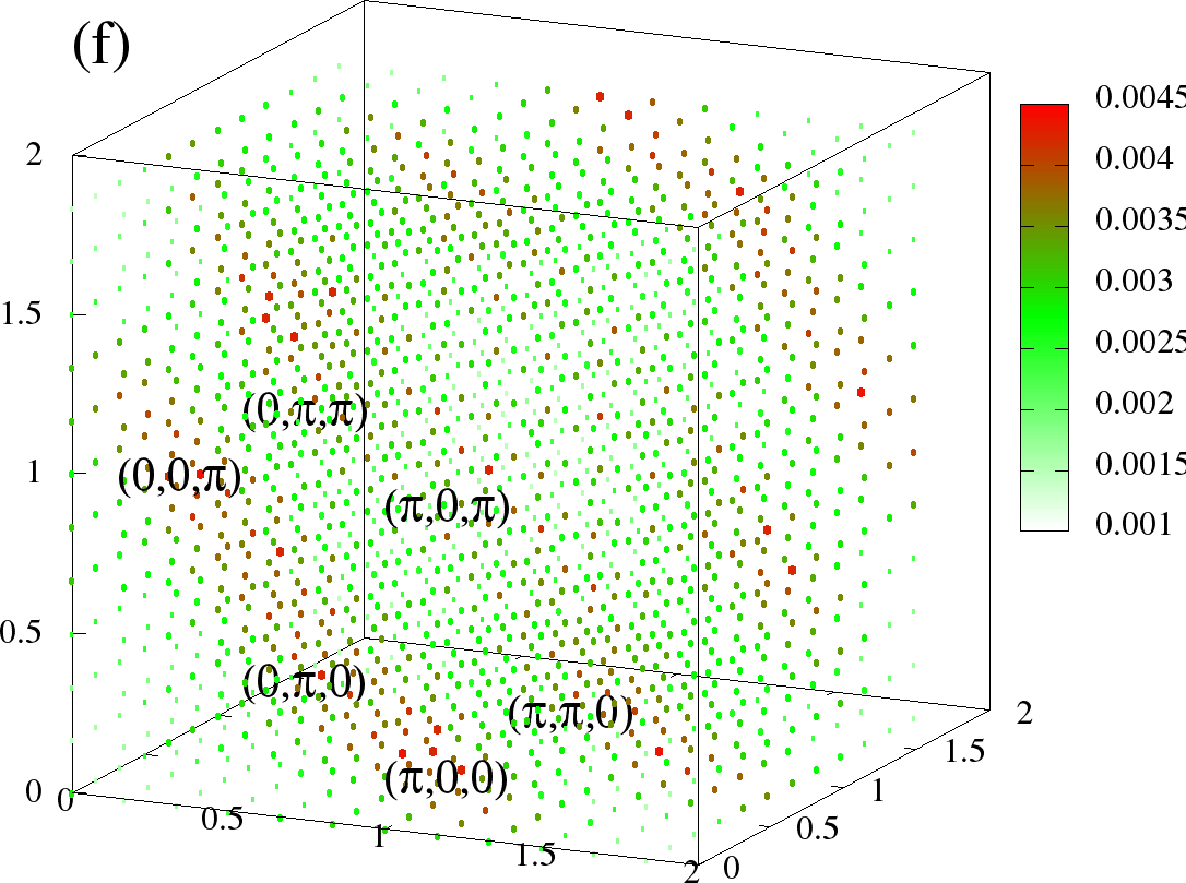 |
Figure 6:The full at (left column) and (right column). The momentum along each axis goes from . (a)-(b) is for FM, (c)-(d) is A-type, and (e)-(f) is for the flux like phase. The densities correspond to the same values as in Figure 5. In these scattered point plots, the colour and the size of the points at given scales with the . The scaling is chosen different for each phase, but same for two temperatures. Because of the specific colour scheme chosen, the low values are small white circles, which are essentially invisible, highlighting only the higher values. In each case (a)-(f), the three axes correspond to ,, respectively, and are in units of , ie., they go from 0 to .
For FM (Figure 6 (a)-(b)), we see two bright spots at and at low temperature, which correspond to the values for ideal ferromagnet (see Table 1). At higher temperature , its weight goes down, but other are still negligible, as the temperature is lower than .
The A-type phase should ideally have peaks at , and , or one of its symmetry related s (Table 2). However, at low temperature, as in Figure 6(c) it has comparable weights corresponding to A and A, and few subdominant neighbouring s. These weight quickly diminish with increasing temperature (Figure 6(d)).
The Figure 6(e) shows the structure factor at density where we expect the flux phase. Here the maximum weight lies close to values corresponding to flux phase (Table 1), but the weight is more dispersed, and there are a lot of sub-dominant s. With increasing temperature, they diminish quickly.
Using the structure factor data, we establish the phase diagram for that is plotted in Figure 7. The Monte Carlo captures mainly three collinear phases, namely FM, A-type, and a phase. The phase corresponds to two FM up planes followed by two FM down planes and so forth. As the carrier density is increased by increasing , we find a FM phase followed by the A-type AF. A phase appears in a thin window surrounded by FM itself. We suspected that this as a finite size effect, and a comparison with the energy of the FM on larger lattices (203), shows that the FM is indeed the ground state in the thermodynamic limit, and so we consider FM and collectively as FM only, and presence of is not indicated in the phase diagram.
Figure 7: diagram for (top to bottom rows) as estimated from the Monte Carlo. Starting from low density () towards high density (), we find FM with high T, thin window of A-type order with very low T compared to FM, followed by the ‘flux’ phase (at ) or ‘spiral’ (at larger ). The symbols are the actual MC estimated T, while the smooth lines are fit to the data.
The FM is stable at the ends of the density window, and its region of occurrence is slowly enhanced as we increase , see Figure 4 as well. The however decreases with increasing since the degree of B-B mixing (and kinetic energy) decreases.
With increase in the 2D system is known to make a transition to a line-like phase, and then a ‘G type’ phase (up spin surrounded by down, etc). The equivalent in 3D would be a progression from FM to a ‘planar’ (A type) phase, then a ‘line like’ (C type) phase and finally to a G type phase if possible. Numerical complexity and the geometric constraint modify the picture as below.
We do access the A type phase with some difficulty but our Monte Carlo cannot access the long range ordered C type phase. However, we see clear evidence of C type correlations in the structure factor. Comparing the energy of the ideal C type phase with the short range correlated phase that emerges from the MC we infer that C type order is indeed preferred over a parameter window. However, we cannot estimate a reliable scale. In the next section we will see the variational results on the C type phase and get a rough estimate of the .
Figure 8:Density of states for the F, A, C, FL (‘flux’) and PM (paramagnetic) phases. (a) and (b) . For both the bandwidth decreases in the sequence: F, PM, C, FL, and A (FL and C have same bandwidth). The plot for is split in two parts, with the region between , with zero weight, omitted. The function arises from the localized B level.
The G type phase is geometrically disallowed on the B sublattice due to its FCC structure. An examination of the structure factor in the density window suggests ‘flux’ like correlations at small which evolves into a spiral at larger . The frustration reduces the of the phases in this density window compared to that of the FM. We can calculate the energy difference between a fully random spin configuration and the variational ground state. This serves as a crude measure of the of the phase.
When , the electron delocalisation happens through B-B-B paths only (see the conduction paths, for example of collinear phases A and C in Figure 3(b) and Figure 3(d) respectively). In this case all the phases have an atomic level located at in the limit . This is directly seen in the density of states (DOS) of these phase. In Figure 8 we show the DOS for the F, A, C, ‘flux’ and paramagnet phases. This dispersionless level gives constant in density region . This feature, and several others, are modified by finite B-B hopping, which leads to broadening of this level. It makes the DOS of the various magnetic phases asymmetric (in energy) and also destroys the particle-hole symmetry in the phase diagram.
2.2Variational scheme
Using the variational scheme discussed earlier one can establish a ground state phase diagram. This is consistent, overall, with correlations that we see in the Monte Carlo, and now allows us to compare candidate phases on large sizes. This establishes the window of existence of the collinear phases, FM, A and C.
For the middle part of the density window no simple phase is suggested by the Monte Carlo. The variational scheme suggests the phases to be SP, SP, SP, and ‘flux’. See the configurations in Figure 3 (e)-(f) and details from Table 1.
The variational scheme also allows a rough estimate of the scale of the ordered state. Ideally, one should compute the energy of ‘spin wave’ configurations about the non trivial ground state, fit these to an effective Heisenberg model, and then work out the of that model. Here we simply compute the ‘binding energy’ of each ordered phase, i.e, its energy gain with respect to the paramagnetic phase at the same electron density, and use the size normalised value as an estimate of .
where corresponds to the variational minimum and to the paramagnet.
This calculation is no substitute for the full MC, and is only meant to supplement the MC based information and provide a rough estimate where MC is noise limited.
Figure 9:The per site energy difference of the variational ground-state and the paramagnetic phase. This provides a rough estimate of the . The parameters are and in all cases. The sequence of phases from low density to middle is FM, A, C and ‘flux’ () or spiral (). The decrease in the ‘T’ with is more drastic in AF phases.
3Results: next neighbour hopping
The model with only ‘nearest neighbour’ (BB) hopping has a rich phase diagram. However, this has the artificial feature of a non dispersive level. In reality all materials have some degree of BB (Sanyal et al. (2009)) hopping due to larger size of B ion, and we wish to illustrate the qualitative difference that results from this hopping. We explored two cases, and for these particle-hole asymmetric cases.
The ground state phase diagram for , obtained by a combination of MC, and variational calculation, is shown in Figure 10 . Turning on has a significant effect on the phase diagram, compare with the case, Figure 4. The particle hole symmetry is destroyed but a reduced symmetry still holds. The phase diagram is richer in the middle of the density window where crossing among various phases occurs at different densities. Due to the symmetry mentioned above it is enough to discuss the case with .
Figure 10:Ground state phase diagram in the presence of .
The A-type phase becomes very thin in the left, but unaffected by , while in right side it widens up in the low and gets replaced by the spiral quickly as we go up in . ‘flux’ and C-type both become stable for high with a gradual shift in the high density. For , at very small in the left and the middle part A-type and the spiral are major candidates with small window for C-AF and ‘flux’. The behaviour in this part is not very sensitive to sign of .
Focusing on , as go up from to the AF phases become less and less stable and are almost wiped out from the left part of the density, and FM becomes stable there. The largest stability window of FM occurs roughly near , where its stable up-to . Going further with higher , FM looses its stability, from C type, ‘flux’ and spirals. However, there is very thin strip of stability of the FM in the band edge in the left part, and towards the middle density, there is re-entrance of the FM phase. In the right part of the density window we have FM, A type and spiral. Increasing reduces the stability of A type to FM, making it vanish near , while FM window keeps increasing with .
Overall, , shows a rich set of antiferromagnetic phases, while , gives a ferromagnetic window, suppressing antiferromagnetic phases.
3.1Monte Carlo
Figure 11: for and at (a): a typical density for A-type phase and (b): a typical density for C type phase. A demonstration of with no sub-dominant peaks, unlike at .
| Low T | High T |
|---|---|
 |  |
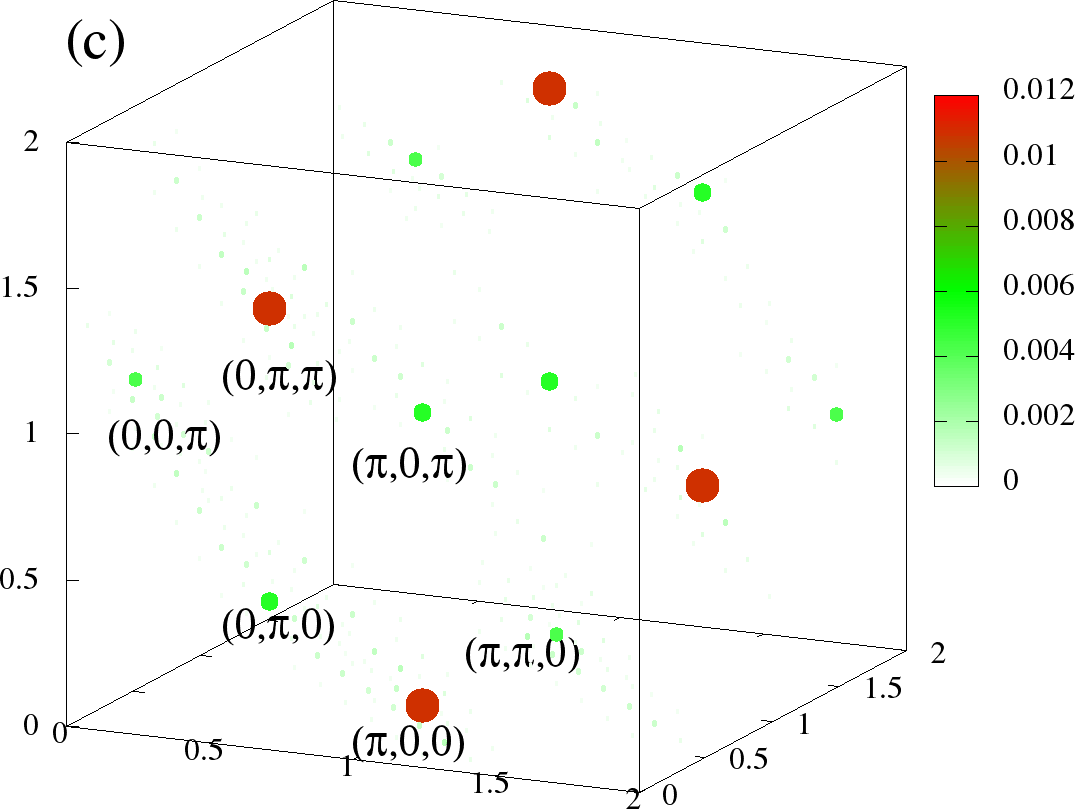 | 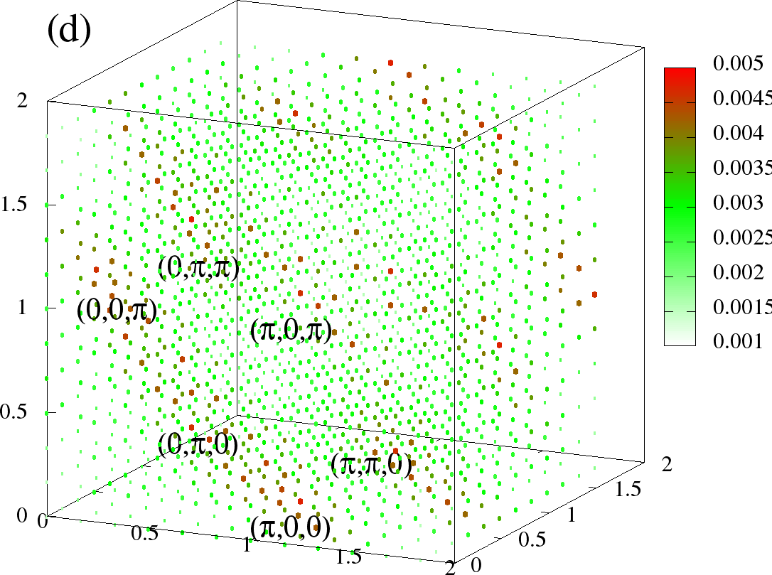 |
Figure 12:The full at (left column) and (right column) (a)-(b) is for A-type, (c)-(d) and is C-type at the same densities as Figure 11. The plotting scheme is same as in Figure 12. The scaling is chosen different for each phase, but same for two temperatures. The visible points denote the dominant values. The three axes correspond to ,, respectively, and are in units of , ie., they go from 0 to .
In Figure 11(a),(b) we show the structure factor data at two densities, for (a) A type and (b) C type phases, to demonstrate one remarkable difference from the particle-hole symmetric case. Figure 12 shows the full structure factor at low (T=0) and some high temperature () at the same densities for A and C type phases.
As we saw earlier in Figure 5 (temperature dependence) and Figure 6 (full ) for the structure factor data were very noisy for AF phases, with many sub-dominant q peaks around the central peak. The saturation value for the A-type peak in the symmetric case was , while now it is , close to the ideal value of 0.25! This is also evident for the full structure factor. Figure 12(a) shows clean peak at and , with other s essentially zero. The largest weights of C-type (Figure 12(c)) are close to and , with very few subdominent s (recall table Table 1 for values of clean phases).
The sharp change in the structure factor makes the identification of the scale more reliable. Although inclusion of does not remove the noise completely, it is reduced over a reasonable part of the phase diagram.
Figure 13(a) presents the phase diagram for and established from Monte Carlo, along with the from the variational approach (Figure 13(b)). In this case, the phases that appear as a function of density are FM, A type, spiral, C type, A type and FM again. For FM, the window of stability gets reduced in the left (low density) part but enhanced in the right (high density) part. The phase appears again, but being a finite size artifact, is absorbed in the FM (and not shown).
The is usually reduced, from the symmetric () case, as hopping provides conduction paths that are non-magnetic. There is a wider space with moderate for A type phase, located asymmetrically in density. It is more stable, in the right window, than left window. The correlations of spiral and C type phases are also captured with relatively less noise, see Figure 11(b) for example of C-type correlation. The phase diagram for and , can be obtained from transformation , i.e., reversing the density axis of Figure 13(a),(b).
3.2Variational scheme
We also used the variational scheme to get an independent feel for the ground state and the for . For the trends from MC are well reproduced by the variational scheme on large systems at \D=0. We observe reduced stability of FM at low density and enhancement at high density.
Figure 13:Phase diagram obtained via Monte Carlo (left) and from the variational calculation (right) at and .
Note that the overall correspondence between the Monte Carlo and the variational approach is much better here than in the case, Figure 7 and the Figure 9.
In Figure 14 we have shown the calculated for 20 size, for . For and (Figure 14(a)-(c)) shows asymmetric (or ), for ferromagnet. The stability windows of the A type is enhanced, the large window of flux phase that was for , is reduced in competition to spiral and C type. For the , (Figure 14(d)) is just density reversed due to symmetry. However, the intermediate (Figure 14(e)) has a large stability window of ferromagnet. Here, though the and are non-zero, due to unusually large stability window, the (or ) is large. For larger (Figure 14(f)), the ferromagnet appears in the middle and right with moderately reduced (or ), while the same is heavily suppressed for antiferromagnetic phases.
Figure 14:Asymmetric case, the energy difference of ground-state and paramagnetic phase. Top: The trends of match with T. Bottom: where FM is stable in the large portion of the density.
To summarize, from the MC and variational data we learn that, apart from asymmetry in the phase diagram, collinear FM and A type phases become stable in wide density window. Their however is slightly reduced than the symmetric case. The S(q) data showing less noise for A, C type and spirals indicates that the energy landscape become ‘smoother’ by so that annealing process becomes easier to get to the ground state. The energy differences as well as MC estimated s show overall decrease with . This is understandable as, by introducing we allow electrons to more on the ‘non-magnetic’ sublattice B. Now the energy of any phase, depends on the energy gain via the hopping process. From the nearest hopping, this gain scales as subject to spin configurations, while the from the next nearest hopping, this gain simply scales as , and doesn’t care upon spin configurations. So more we increase and , the more we are making the energy of the system insensitive to spin-configurations. The asymptotic limit of this is when every phase has same energy as paramagnet.
In the couple of paragraphs below we try to create an understanding of how the phase diagram is affected by . Unfortunately we do not understand the effects over the entire density window yet.
For , the FM loses its stability to AF phases even at low . That is puzzling since one would expect the FM phase to have the largest bandwidth. We recall that in the case, there is a localized band coming from B level for all the phases. The dispersion of this previously localized level causes the and to have a dependent separation, which was for all in the symmetric case. The separation for these levels in the asymmetric case is , which varies from , to in 3D. In 2D it varies from from , to . Figure 15 shows the lowest eigenvalues of F,A,C and flux phases with for and we see how a crossing occurs at .
Figure 15:Asymmetric case, lowest eigenvalues plotted as function of for the F,A,C and flux phases calculated from the dispersions. (a) and (b) .
We make a general observation about the change in the ‘energy landscape’ of the model, in the space of spin configurations, with changing . If then the electrons could delocalize on the wide based band populating the non magnetic sites only. Magnetic order would make little difference to electronic energies and the energy landscape would be featureless. There are no ordered states as minimum in this landscape. Contrast to , where delocalisation takes place necessarily through the magnetic sites and deep minima in in the landscape represent ordered states in real space. There are presumably shallow metastable states possible too.
At intermediate the ordered states are shallower, since the gain from magnetic ordering is lower, but the metastable seem to be affected even more, if the relative ease of Monte Carlo annealing is any indicator.
4Discussion
The real double perovskites are multi-band materials, involving additional interaction effects and antisite disorder beyond what we have considered here. Nevertheless, we feel it is necessary to understand in detail the phase diagram of the `simple’ model we have studied, and then move to more realistic situations. In what follows, we first provide a qualitative comparison of the trends we observe with experimental data, and then move to a discussion of issues that are ignored in the present model.
4.1Comparison with experiments
There is limited experimental signature (Jana et al. (2012)) of metallic AF phases driven by the kind of mechanism that we have discussed. So, the comparison to experiments is, at the moment, confined to the scales (Navarro et al. (2001), Park et al. (2009)) etc, of the ferromagnetic DP’s.
From the ab initio calculations (Sanyal et al. (2009)) the sign and , so one can compare the right panel of Figure 4 qualitatively with experiments.
In a material like SFMO the electron density can be increased by doping La for Sr, i.e., compositions like SrLaFeMoO. This was tried (Navarro et al. (2001)) and the increased from 420K at to 490K at . SFMO has threefold degeneracy of the active, , orbitals while we have considered a one band model. When we create a correspondence by dividing the electron count by the maximum possible per unit cell (3 in our case, 9 in the real material), in our units corresponds to and to .
When , as a function of the peaks around , Figure 7, quite far from the experimental value. However, in the presence of and , Figure 14(e), the peak occurs above . So, modest can generate the ferromagnetic window that is observed, and produce a . For eV, this is in the right ballpark.
Ray et al experimentally estimate the onset of AF order upon La doping to be , which corresponds to . Our onset of AF order, for \D in [0-10], is , which for SFMO would be . This is quite close to experiments. However, inclusion of finite , pushes this to lower values.
4.2Additions to the model
(i)~Effect of orbital variables: Apart from renormalization of the electron count, multiple orbitals could, in principle, have a qualitative effect. If the local orbital degeneracy is lifted by Jahn-Teller effect then the resulting ‘orbital moment’ could order in some situations. This orbital ordered (OO) background can modify electron propagation and the magnetic state. This is known to happen at some dopings in the manganites. Even there, however, the broad sequence of magnetic phases is consistent with predictions from a one band model. The double perovskites do not seem to involve strong lattice effects, the orbital degeneracy survives, and there is no orbital order. This suggests that there is even better chance of a one band model being qualitatively correct here, compared to the manganites.
Had there been strong OO effects, the spin-spin coupling in that background may have picked up strong directionality, and the geometric frustration could have been irrelevant. This does not seem to happen in most double perovskites. Indeed, there are experiments on the insulating DP’s (Wiebe et al. (2002), Aharen & others (2010), Aharen & others (2009)) where the geometric frustration of the FCC lattice leads to a non trivial magnetic state, unrelieved by the presence of multiple orbitals.
We of course expect that the phase boundaries and scales that we calculate would be affected by the orbital degeneracy. However, the trends in the phase diagram with increasing density simply reflect a growing AF tendency and the non coplanar phases emerge due to the impossibility of Neel order.
(ii)~Antisite disorder: Attempts to increase via A site substitution also brings in greater antisite disorder (B-B interchange) and even the possibility of newer patterns of A site ordering (!) complicating the analysis. For example, one would try compositions of the form: AABBO, where A and A have different valence in an attempt to change . The assumption is that the A only changes without affecting other electronic parameters, i.e., A ions do not order and remain in an alloy pattern. This may not be true. In fact, at , the material AABBO may have a specific A-A-B-B ordering pattern that affects electronic parameters in a non trivial way and one cannot understand this material as a perturbation on ABBO. In such a situation one needs guidance from experiments and ab initio theory to fix electronic parameters as is varied. All this before one even considers the inevitable antisite (B-B) disorder and its impact on magnetism (Singh & Majumdar (2011)).
## Conclusions
We have studied a one band model of double perovskites in three dimensions in the limit of strong electron-spin coupling on the magnetic site. The magnetic lattice in the cubic double perovskites is FCC and increasing the electron density leads from the ferromagnet, through A and C type collinear antiferromagnets, to spiral or ‘flux’ phases close to half-filling. We estimate the of these phases, via Monte Carlo and variational calculation. The introduction of BB hopping significantly alters the phase diagram and scales and creates a closer correspondence to the experimental situation on DP ferromagnets.
- Sanyal, P., & Majumdar, P. (2009). Phys. Rev. B, 80, 054411.
- Kumar, S., & Majumdar, P. (2006). Eur. Phys. J. B, 50, 571.
- Alonso, J. L., Capitán, J. A., Fernández, L. A., Guinea, F., & Martín-Mayor, V. (2001). Phys. Rev. B, 64, 054408.
- Fazekas, P. (1999). Lecture Notes on Electron Correlation and Magnetism. World Scientific.
- (N.d.).
- Sanyal, P., Das, H., & Saha-Dasgupta, T. (2009). Phys. Rev. B, 80, 224412.
- Jana, S., Meneghini, C., Sanyal, P., Sarkar, S., Saha-Dasgupta, T., Karis, O., & Ray, S. (2012). Phys. Rev. B, 86, 054433.
- Navarro, J., Frontera, C., Balcells, L., Martinez, B., & Fontcuberta, J. (2001). Phys. Rev. B, 64, 092411.
- Park, B.-G., Jeong, Y.-H., Song, J. H., Kim, J.-Y., Noh, H.-J., Lin, H.-J., & Chen, C. T. (2009). Phys. Rev. B, 79, 035105.
- Wiebe, C. R., Greedan, J. E., Luke, G. M., & Gardner, J. S. (2002). Phys. Rev. B, 65, 144413.
- Aharen, & others. (2010). Phys. Rev. B, 81, 064436.
- Aharen, & others. (2009). Phys. Rev. B, 80, 134423.
- Singh, V., & Majumdar, P. (2011). Eur. Phys. J. B, 83, 147.